the Creative Commons Attribution 4.0 License.
the Creative Commons Attribution 4.0 License.
 | 29 Sep 2022
A review of different mascon approaches for regional gravity field modelling since 1968
Markus Antoni
The geodetic and geophysical literature shows an abundance of mascon approaches for modelling the gravity field of the Moon or Earth on global or regional scales. This article illustrates the differences and similarities between the methods, which are labelled as mascon approaches by their authors.
Point mass mascons and planar disc mascons were developed for modelling the lunar gravity field from Doppler tracking data. These early models had to consider restrictions in observation geometry, computational resources or geographical pre-knowledge, which influenced the implementation. Mascon approaches were later adapted and applied for the analysis of GRACE observations of the Earth's gravity field, with the most recent methods based on the simple layer potential.
Differences among the methods relate to the geometry of the mascon patches and to the implementation of the gradient and potential for field analysis and synthesis. Most mascon approaches provide a direct link between observation and mascon parameters – usually the surface density or the mass of an element – while some methods serve as a post-processing tool of spherical harmonic solutions. This article provides a historical overview of the different mascon approaches and sketches their properties from a theoretical perspective.
- Article
(2601 KB) - Full-text XML
- BibTeX
- EndNote


The gravity field of the Earth influences daily life in many ways. Local plumb lines define the upward direction, and several scientific instruments must be levelled before usage. Gravity measurements provide corrections for geophysical height systems and allow the exploration of mineral deposits or caves. A gravity field model is also required for inertial navigation systems within aeroplanes, ships or submarines. On a regional or global scale, mass redistributions – like the melting of glaciers or the changes in ground water – are reflected in the temporal variations of the gravity field.
The gravity field of the Earth – or another celestial body – can be analysed on a global scale when enough orbiting satellites are tracked, even without special onboard instruments or ground-based measurements. Satellite data provide a fast and homogeneous sampling in contrast to ground-based observations. The gravity field analysis establishes a connection between the tracking data and a set of base functions to model the gravity field. An analysis by spherical harmonic functions is preferable for spherical bodies, as these base functions are the natural solution of the Laplace equation. This set of base functions is also a complete and orthogonal system, which simplifies the analysis. However, a reasonable spherical harmonic analysis requires orbit observations with global and homogeneous data distribution, and the model will have the same resolution everywhere.
Alternative localising base functions – e.g. point masses, spherical radial base functions, wavelets, Slepian function – are investigated and applied when the data distribution is irregular or when more details in a region of interest shall be detected. This article will summarise the localising base functions, which are labelled as mascons and applied for the gravity field modelling of the Earth and Moon.
Studies of the early lunar orbiters demonstrated significant orbit disturbances, which were traced back to an irregular lunar gravity field. The term “mascon” was introduced by Muller and Sjogren (1968b) for describing these mass concentrations near the surface. In the same work, the name mascon was also introduced for the mathematical modelling of these mass concentrations. The concept was applied for several years to the gravity field of the Moon, as the method was capable of the nearside restriction of data in contrast to spherical harmonic solutions. Interest in regional modelling of the Earth's gravity field has increased significantly since the gravity field mapping mission GRACE (2002–2017) and its successor mission GRACE-FO (2018–present). The new observations enabled the analysis of temporal variations caused by the redistribution of water and ice masses, where regional gravity field modelling overcomes the spherical harmonic solutions. Hence, the mascon concept has been adapted and applied to Earth-related data by several research groups, either for regions of interest (Luthcke et al., 2008; Schrama et al., 2014; Ran et al., 2018) or on a global scale (Koch and Witte, 1971; Andrews et al., 2015; Save et al., 2016).
A closer inspection of the publications, however, shows a variety of approaches under the label of mascons. This article will give a historical overview of the most prominent representatives and an adequate definition of the mascon base functions. All different meanings of the investigated mascon approaches can be covered by the following definition: the term mascon either refers to the fact of a significant gravitational anomaly within a celestial body or to a modelling of these anomalies by localising base functions. The localising base functions, which are labelled as mascons, include point masses or discrete surface elements based on the simple layer potential. In the case of surface elements, the surface density is constant per mascon, and each localising base function is – in a spectral representation, at least in the limit of high-degree expansion – a two-dimensional step function on the sphere. Methods of post processing are also labelled as a mascon approach when their surface elements have a constant surface density. The shape of the mascon is not relevant for the definition, and the surface of the celestial body is not necessarily covered.
This publication is focused on the mascons' definitions and will ignore other processing steps, like background models, regional constraints or regularisation techniques. Each mascon approach is presented by the associated gravitational potential of a single element and its gradient in the notation of representative literature. The properties of each approach are deduced from the theoretical perspective only, but without treating programming experiments or numerical aspects. Such a detailed and comprehensive review of the different mascon approaches cannot be found in literature to our knowledge.
In several previous articles, the authors quote only the original publication (Muller and Sjogren, 1968b) for the term mascon and restrict themselves in the following texts to a specific mascon approach with its literature (e.g. Luthcke et al., 2008; Lemoine et al., 2007; Krogh, 2011; Andrews et al., 2015).
A point mass model and planar discs are applied for modelling the lunar gravity field in Wong et al. (1971), and both methods are considered as mascon approaches. In Watkins et al. (2015) and Save et al. (2016), different mascon approaches are presented in the introductions, but without formulas or historical background. The authors of both articles classify three principal concepts:
- A.
mascons that have an analytical expression for the gravitational potential and explicit partial derivatives for the gradient;
- B.
mascons that are represented by a finite series of spherical harmonic functions and with partial derivatives derived via the chain rule;
- C.
mascons that serve as a post-processing tool to obtain regional mass changes from monthly spherical harmonic solutions.
An analogous classification with additional literature is presented by Abedini et al. (2021a), whose contribution is a numerical method for the gradient, which does not fit into the threefold scheme.
Many recent publications are related to the mascon solutions of either the NASA Goddard Space Flight Center (GSFC), the Jet Propulsion Laboratory (JPL) or the Center for Space Research (CSR). The current JPL solutions are spherical cap mascons with analytical partial derivatives – i.e. category A in the classification – which are presented in Sect. 3.2. The mascon approaches of GSFC and CSR are based on spherical harmonic functions, and they are a prominent example of type B (see Sect. 3.1). The mascon visualisation tool at the University of Colorado Boulder (https://ccar.colorado.edu/grace/index.html, last access: 23 September 2022) enables an analysis and comparison of the latest solutions at JPL and GSFC for regions and generates time series per location.
2.1 Mascons – mass anomalies close to the Moon's surface
The origin of the mascon concept is closely related to early models of the lunar gravity field.
In the space race between the Soviet Union (USSR) and the United States of America (USA), both nations wanted to send their representatives to the Moon first. The possible landing sites were investigated by spacecrafts, starting with Luna 1 (USSR) in 1959, which missed the Moon due to navigation issues. The first man-made object on the Moon was the space probe Luna 2 (USSR) in a design impact in 1959, followed by several missions by both nations. The spacecraft Luna 10 (USSR) and Lunar Orbiter 1 (USA) were the first artificial orbiters around the Moon in 1966 (Neal, 2008).
In both orbiter missions, the observed orbits differed after a short time from the predicted ones, which indicated either an incorrect or an incomplete model. As other error sources could be excluded soon, the orbit disturbances were explained by significant mass anomalies below the Moon's surface. For these anomalies, the term “mass concentration” or “mascon” was introduced in Muller and Sjogren (1968b).
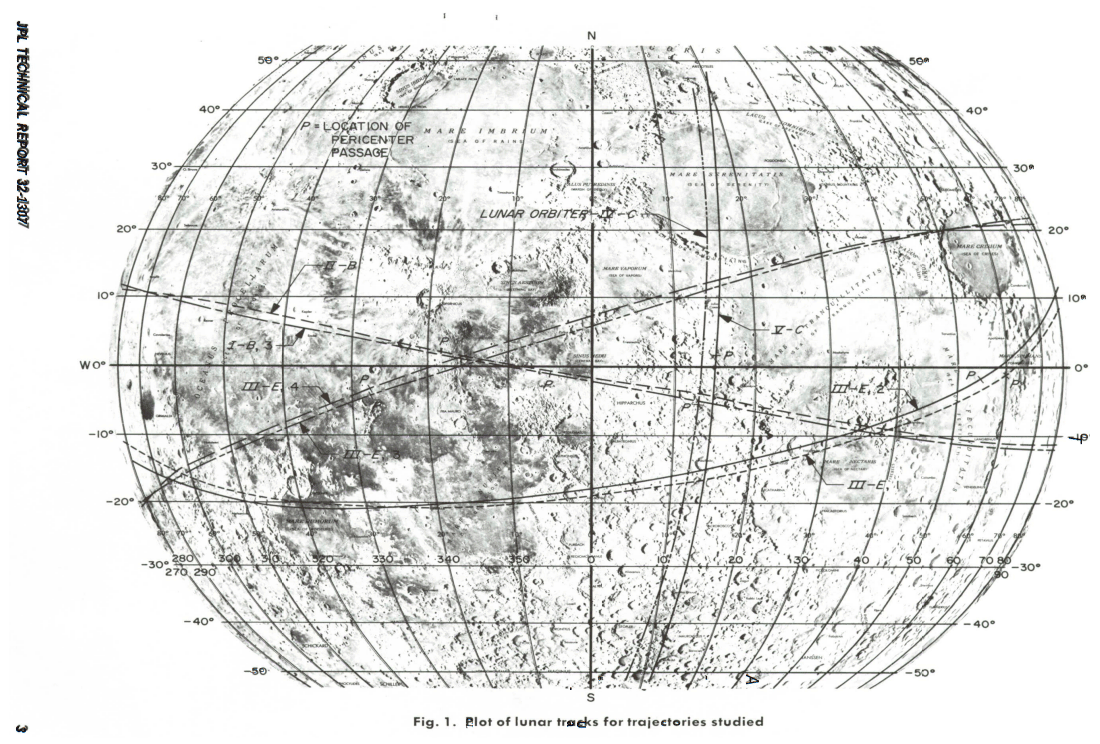
All identified mascons on the nearside of the Moon cause relatively large and positive effects up to 200 mGal, and their locations are one-to-one correlated to the major lunar maria, including Imbrium, Serenitatis, Crisium, Humorum and Nectaris, which are visualised in Fig. 1 (Muller, 1972).
In particular for the Moon it is still common to call a large area with a significant positive mass anomaly a mascon independent of its mathematical representation (Floberghagen, 2001, p. 3). A similar behaviour can be found, for example, in Barthelmes (1986, p. 35), where the mass anomalies of the Earth's gravity field are called mascons without using the phrase for the mathematical modelling as well. This thesis focuses on the point mass modelling, but it also sketches simple layer potential with discrete surface elements, and both aspects will be identified as mascon approaches in the current article.
2.2 Point mass mascons
A quick modelling of the mass anomalies was important for the preparation of the latter space missions and the landing on the Moon. The chosen representation should
-
consider the geographical pre-knowledge, i.e. the lunar maria as expected locations of the mass anomalies;
-
consider the observation geometry, i.e. the fact that only the near side of the Moon allows observations from terrestrial ground stations;
-
enable a direct relation between observables – Doppler tracking data in the case of the early lunar missions – and the estimated mascon parameters;
-
remain simple due to limited computer resources.
The first three requirements are still important arguments for regional gravity field analysis – by mascons, wavelets, radial basis functions, Slepian functions, etc. – while the limited resources implied a simple modelling of the anomalies by point masses.
The original papers (Muller and Sjogren, 1968a, b; Muller, 1972) lack a formula representation of the potential, but it is re-constructed, for example, in Floberghagen (2001, p. 19):
with
-
V(rP): gravitational potential at the calculation point rP;
-
G: gravitational constant;
-
M: mass of the celestial body;
-
δmq: mass ratio between point masses and total mass M;
-
rq: centres of the point masses.
Please note that, for consistency, all mascon quantities and their geometries are labelled in this article by means of an index (here: ), and the calculation point is labelled by the index P, both independent of the cited articles.
2.2.1 Relation to the observation and the estimation process
A standard observation technique for space probes is the Doppler tracking, i.e. the change in frequency of a (re)-transmitted signal due to the relative motion of the spacecraft and the ground station. The American missions use a few globally distributed stations, which meanwhile form the Deep Space Network of the NASA and which are operated by JPL today1. The Doppler signal does not provide complete information on the position or velocity; rather, it only projects the relative velocity between station and space probe onto the line of sight (Muller and Sjogren, 1968a; Weinwurm, 2004; Floberghagen, 2001).
The relationship between observation and mascon parameters requires a description of the change in the velocity – i.e. the acceleration – of the spacecraft caused by the gravitational potential. Hence, it is sufficient to derive the gradient by of the potential. For point mass models, the gradient is calculated via
To emphasise the special requirements and restrictions for the early lunar modelling, some details will be sketched here as well: according to Muller and Sjogren (1968a, b), residual observations are created by removing the gravitational effect of a tri-axial Moon model and the acceleration of the Sun and other planets from the raw Doppler tracking data. Cubic polynomials are fitted to the residuals for smoothing and estimation of accelerations. The accelerations are mapped to a constant orbit height of 100 km altitude above the Moon's surface. The point masses are introduced directly below the trajectory, with a depth of 50 km below the surface, and their magnitudes are estimated. Additional information is given in Wong et al. (1971), such as the restriction to 100 parameters in the estimation process due to implementation as well as the step-wise solutions in north–south bands, which usually cover 8 trajectories – with 48 elements in the estimated state vectors – and around 50 point masses below the tracks.
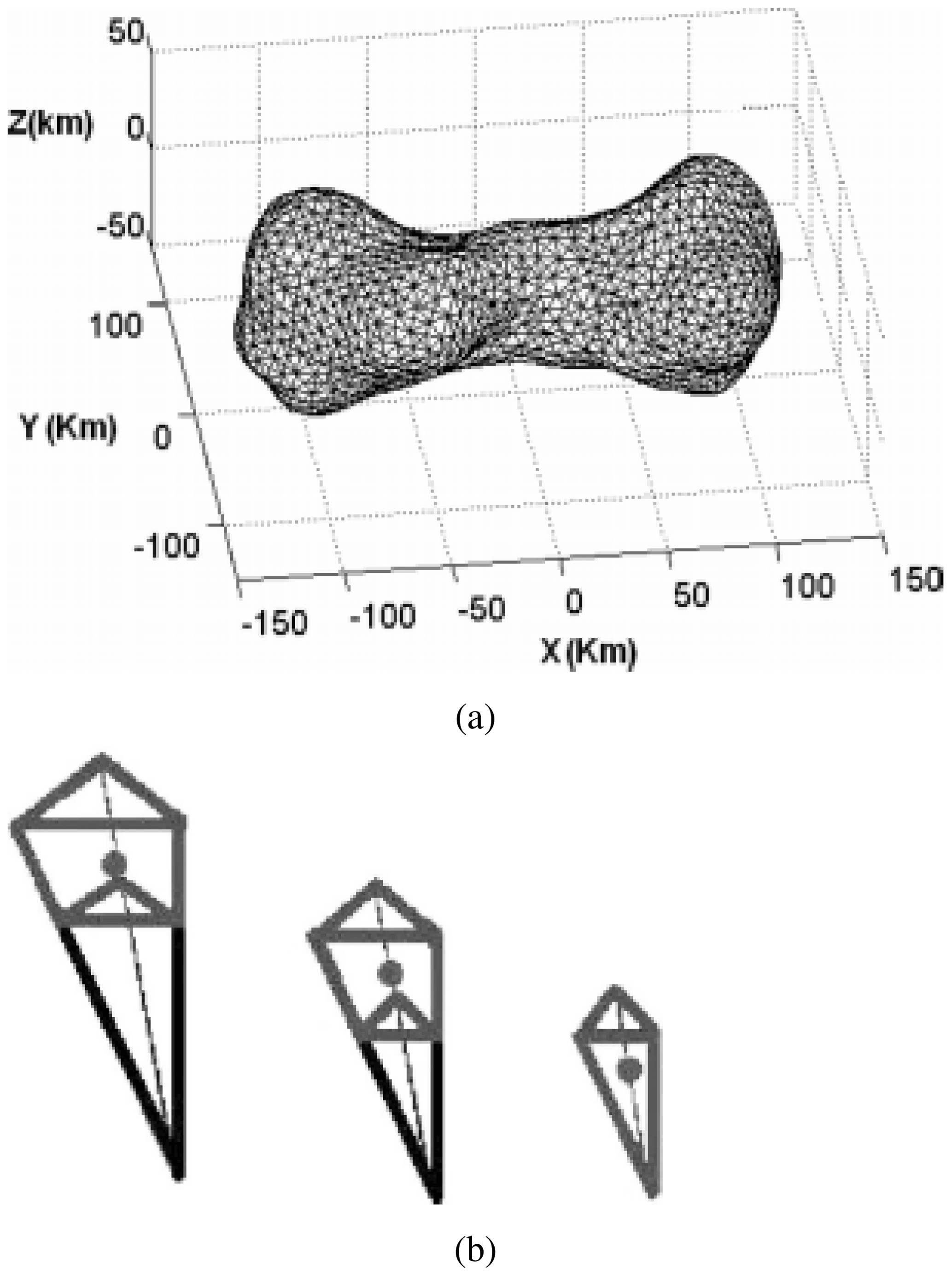
Figure 2Modelling the gravity field of the asteroid 216 a.k.a. Kleopatra by point mass mascons according to Chanut et al. (2015). (a) Polyhedron model of the asteroid; (b) geometrically sub-division of one tetrahedron by parallel planes with the mascon locations as large dots. Panel (b) was converted to grey-scale for this article.
2.3 Point mass mascons for irregular celestial bodies
Point mass mascons are also used in a different way to determine the gravity field of irregular celestial bodies. An example can be found in Chanut et al. (2015), where the gravity field of the asteroid 216 – also known as Kleopatra – is predicted by polyhedron models and point mass mascons. In the case of asteroids, the irregular shape is observed by optical instruments first; only in rare cases, orbiters investigate the gravity field directly. The observed shape is approximated by tetrahedrons with three corners on the surface and one in the geometrical centre of the asteroid (see Fig. 2a). Point masses are located then, either one per tetrahedron in its geometrical centre or three in the centres of a geometrically sub-divided tetrahedron (see Fig. 2b). Assuming a constant density of the asteroid and a known total mass, the mass per mascon is assigned to a value proportional to the surrounding volume, and the gravity field around the object can be predicted.
Properties
The point mass mascons have closed formulas for potential and explicit partial derivatives, which identify them as type A mascons in the threefold scheme.
- +
-
The method is very easy to implement and requires only a few computational resources.
- +
-
The gradient and all other field quantities are found without quadrature.
- −
-
The model is singular for the potential and the gradient at the location of the point masses.
- −
-
In the case of the lunar gravity field, assumptions are required for the location and depth below ground, as the Doppler tracking data and the observation geometry do not allow a detection of this information from the measurement.
It should be pointed out that the modelling by point masses is applied, for example, in Baur and Sneeuw (2011) or in Barthelmes (1986), Claessens et al. (2001), and Lin et al. (2014) without being labelled as a mascon approach by the authors, and that in the latter examples also the positions of the masses are estimated for regional studies of the Earth's gravity field. An iterative algorithm is developed and justified via quasi-orthogonality in the sense of an inner product in Barthelmes (1986). To stabilise the optimisation process, the possible movement per point mass shall be restricted in depth but also in radial or tangential direction with respect to an initial position.
2.4 Planar disc mascons
As a response to Muller and Sjogren (1968b), an article by Conel and Holstrom (1968) presented a physical interpretation of the ringed lunar maria, according to which former impact craters are filled afterwards by denser material. The authors experiment in the modelling of the mass anomalies with an arrangement of planar discs of finite thickness inside the impact craters and demonstrate a better post-fit to the residual Doppler tracking data for Mare Serenitatis.
The obvious issues of point masses are discussed in Wong et al. (1971):
-
the singularities of the model at the centres;
-
bad fitting of the residual tracking data in the equatorial zone of the Moon due to the observation geometry;
-
and combination issues with the spherical harmonic models (of very low degree and order at the time).
To overcome these problems, finite mass elements are suggested for modelling the gravitational anomalies, which also agrees with the physical ideas in Conel and Holstrom (1968).
For a simple and efficient solution, the finite mass elements are chosen to be oblique rotational ellipsoids, also known as spheroids (Wong et al., 1971). The gravitational potential of a spheroid and its gradient are derived in Moulton (1960, pp. 119–132). On the one hand, the gravitational potential requires a series expression:
with
-
M: total mass of the spheroid (the gravitational constant is neglected in this exercise of the book);
-
: Euclidean distance between the spheroid's centre and the calculation point; outside the body,
-
b: semi-minor axis of the spheroid (and semi-major axis a);
-
numerical eccentricity.
On the other hand, the gradient of the potential can be derived in a closed formula. In Wong et al. (1971), the semi-minor axis b is then squeezed to zero, which leads to the attraction of a circular and planar disc. The article provides the gradient of a single disc in the form
where k fulfils the quadratic equation
To bring the expressions of the gradient in Moulton (1960) and Wong et al. (1971) into an analogous form, the identity must be kept in mind. It also turns out that the value k is linked to the numerical eccentricity of the spheroid by the relation .
These planar disc mascons must be rotated and translated on the surface or close to it onto different locations, which is only implicitly indicated due to the definition of the coordinates with respect to the centre of each disc (Wong et al., 1971).
Properties
The planar disc mascons have closed formulas for explicit partial derivatives of the potential, which identifies them as type A mascons.
- +
-
The closed formulas do not require any integration for the gradient.
- +
-
The surface elements all have the same shape, size and area for each mascon.
- −
-
The potential of a mascon requires a series expansion.
- −
-
The model is singular for the potential at the centre of the disc.
- −
-
The surface elements do not cover the complete surface, even in a global analysis.
- −
-
Most points within a disc are either above or below the spherical surface.
In fact, the planar disc mascons are a kind of a simple layer potential, but without implicit or explicit integration for the gradient.
Modelling the gravitational potential by a simple layer was well known in geodesy and became popular around 1970.
The method can be applied to the complete potential or to a residual field after subtracting a reference field. The basic idea is to condensate the (remaining) in-homogeneous mass distribution onto the surface 𝒮, either the topography itself or a simpler reference like a sphere or spheroid (Koch and Witte, 1971; Morrison, 1971).
The gravitational potential of the layer is given by
with
-
V(rP): gravitational potential at the calculation point rP;
-
σ(Ω): location-dependent surface density;
-
G: gravitational constant;
-
:
Euclidean distance2 between calculation point and all surface points , with P∈𝒮; -
dΩ: the differential surface element.
In the mascon version of the simple layer potential, the surface 𝒮 is sub-divided into smaller regions 𝒮q – which are called surface elements or patches in this article – where the density is assumed to be constant. This leads to the mascon representation of the (residual) potential:
A linear combination Eq. (8) of all mascons – where the summation weights σq are included in the potential Vq(rP) per mascon – generates the potential of the simple layer again. On the one hand, it should be pointed out that the method is applied, for example, in Koch and Witte (1971) without being labelled as a mascon approach. On the other hand, all the following mascon approaches are based on the simple layer potential with discrete surface elements and constant surface densities, which justifies the mascon label here.
3.1 Lumped spherical harmonics as mascons
Solving the Laplace equation in spherical coordinates leads to the spherical harmonic functions as a natural basis for gravity field modelling. An adequate linear combination of spherical harmonic functions can also be used to define localising base functions like the mascons in the spectral domain. Due to this combination over all degrees and orders, the result is sometimes labelled as the “lumped spherical harmonic approach” (Klosko et al., 2009).
Firstly, the gravity field is decomposed into a static field and its temporal variations:
The static field and the mascons are represented by spherical harmonic synthesis. According to Heiskanen and Moritz (1967), Koch and Witte (1971) and Seeber (2003), the potential is given by
with
-
: potential of the static field;
-
: spherical coordinates of the evaluation point rP, i.e. longitude λP, co-latitude θP and radius rP;
-
GM: product of gravitational constant G and the mass of the celestial body M;
-
R: radius or semi-major axis of the spherical or ellipsoidal reference body;
-
: fully normalised Legendre functions;
-
: fully normalised spherical harmonic coefficients, also known as Stokes coefficients.
The approach arose at GSFC when analysing the data of the GRACE mission, and it is presented in a sequence of articles (Rowlands et al., 2005; Lemoine et al., 2007; Klosko et al., 2009; Rowlands et al., 2010; Luthcke et al., 2013).
The mascons are generated in the spectral domain by (time-dependent) delta Stokes coefficients or differential Stokes coefficients of a simple layer:
with the Love numbers for considering the loading effects of the extra masses on the surface.
The mascon solutions of the JPL are published online (https://earth.gsfc.nasa.gov/geo/data/grace-mascons, last access: 23 September 2022); the mascon solution of the CSR can also be found online (http://www.csr.utexas.edu/grace/, last access: 23 September 2022). As the formulas require standard techniques of geoscience, other groups are also working with these kind of mascons (e.g. Andrews et al., 2015; Krogh, 2011).
The lumped spherical harmonic approach can be used for any (almost spherical) body, but the approach is introduced for analysing the temporal variations of Earth's gravity field due to the variable water storage in particular. Taking into account that a uniform layer of 1 cm fresh water within an area of 1 m2 has a mass of around 10 kg, the density is re-written in Rowlands et al. (2010) and Luthcke et al. (2013) as σq=10Hq – in Save et al. (2016) the factor σq=10.25Hq is used instead – to express the results in centimetres of equivalent water height. Each mascon is determined by a spherical harmonic synthesis
on the spherical surface r=R and with the upward continuation term in the synthesis formula, if necessary.
If the maximum degree L of the expansion is large enough, expression Eq. (12) forms a “two-dimensional step function” on the sphere 𝒮 (see Fig. 3), with
A straightforward sub-division of a sphere is given by a longitude–latitude grid, i.e. all boundaries are either part of parallel circles or of meridians. In this case, the integrals Eq. (11) have the differential surface element dΩ = cos θdθdλ of the unit sphere, and the integration can be obtained by recursion formulas of integrated Legendre functions.
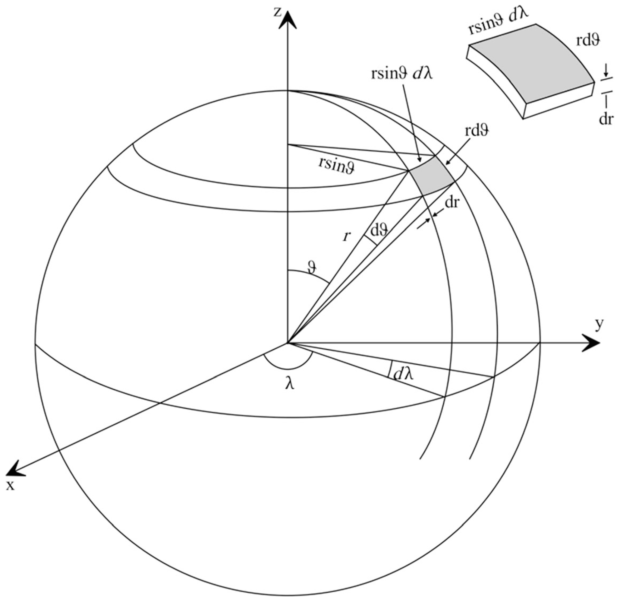
Figure 3Sub-division in a longitude–latitude grid and a differential volume element of the sphere (Abedini et al., 2021a). In an alternative interpretation, the figure illustrates a two-dimensional step function on the sphere, which is either zero (white) outside and constant but non-zero (grey) inside a mascon element.
The size and shape of the surface elements vary between the publications:
-
Lemoine et al. (2007) and Rowlands et al. (2005) present a separation of the region of interest into surface elements of equal angles with the dimension , while Krogh (2011) defines patches of the dimensions and .
-
Equal areas within a longitude–latitude grid can be obtained by stretching or shrinking one of the angles dependent on latitude, which is discussed already in Morrison (1971) and applied in experiments of Rowlands et al. (2010) and Andrews et al. (2015).
-
In Klosko et al. (2009), the surface elements have – at least in the corresponding Fig. 4 – more complex boundaries. The lines are still along parallel circles and meridians, but they are combined in such a way that the mascon patches fill irregular shapes of sub-basins within the Mississippi basin.
-
In the CSR solution, the equal area per mascon is considered to be more relevant than a simple sub-division or a complete coverage of the sphere (Save et al., 2016). A geodesic grid with 40 962 vertices is generated by iteration, and the mascon patches are located in the centres. The shapes of the patches are either hexagonal or pentagonal, and the elements cover approximately equal areas of around 1∘ diameter.
The regularisation techniques for equiangular patches are discussed in Abedini et al. (2021b) for other types of mascons, but the final recommendation to consider herein the area size should be transferable to the lumped spherical harmonic approach as well.
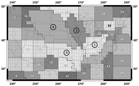
Figure 4Definition of mascon surface elements in the Mississippi basin. The figure originates from Klosko et al. (2009), but it is converted to grey-scale for this article.
Observation of GRACE
The mascons were introduced for analysing the Earth's gravity field in the mission GRACE (Gravity Recovery And Climate Experiment). The mission consisted of two identical satellites, which were launched in 2002 in a cooperation between NASA/JPL and the German DLR. The satellites fell around the Earth in one common and almost circular orbit, with a low altitude of originally 500 km in height. The positions were quasi-permanently observed by GPS receivers with three antennas, and onboard accelerometers with three axes were measuring the combined influence of all non-gravitational effects. The main observable was the variation of the distance between the two GRACE satellites, measured by microwaves in the K-band and Ka-band via a range-rate measurement system. The distance of ρ≈250 km between the satellite centres varied due to mass variations below, and the K-band provided a nominal accuracy of 10 µm for the range ρ and 0.5 µm s−1 for the range-rate (Seeber, 2003; Tapley et al., 2004).
The orbit observations and the gravity field parameters can be linked in different ways – e.g. the variational equation, the energy balance approach, the short arc approach or the acceleration approach – which are sketched, for example, in Liu (2008). The details are not in the focus of this work, but most methods require the gradient of the gravitational potential again.
Gradient of the lumped spherical harmonic mascons
For the range-rate in the lumped harmonic approach, the relationship is found in Luthcke et al. (2013) by the chain rule
and analogously for range-acceleration . The derivatives are straightforward, as the formulas Eq. (11) are linear with respect to the surface density σq or the water height Hq.
Properties
The lumped spherical harmonic approach is a representative of the type B mascons.
- +
-
The method is very easy to implement after a previous analysis of the GRACE observations by spherical harmonic functions.
- +
-
After the determination of all delta Stokes coefficients, all other field quantities can be calculated by standard methods of spherical harmonic synthesis.
- +
-
The required integration Eq. (11) can be solved by well-known recursion formulas or by numerical quadrature.
- −
-
A high degree L of expansion might be required for straight boundaries and constant values within the two-dimensional step functions.
3.2 Spherical cap mascons
The planar disc mascon approach (in Sect. 2.4) is not satisfying from a geometrical view point, as most points within the element are either above or below the spherical surface. This can be avoided by introducing spherical caps instead of planar discs. Monthly solutions in terms of spherical cap mascons are calculated at the JPL, and the details can be found in Watkins et al. (2015).
To reduce the effort of quadrature for the gradient expression, a local mascon coordinate system is introduced for each element by rotation, where the centre of the mascon is equal to the new North Pole of the system. The new coordinates are the spherical distance γ and the azimuth ξ in the calculation point. The potential is still based on the simple layer theory leading to the integral
for the potential of a spherical cap, with
-
: gravitational potential per mascon in the local mascon coordinate system (the over-bar is introduced here to emphasise the rotated coordinate system);
-
σq: product of the gravitational constant G and mass per mascon mq divided by the area of the spherical cap, i.e. ;
-
R: radius of the spherical reference model;
-
ℓ(Ω,rP): distance between calculation point and the points in the spherical cap (in the original paper, the Euclidean distance is noted down by d);
-
α: radius of the spherical cap in radians.
Gradient of the spherical cap mascons
The gradient of the potential is calculated per mascon and rotated at the end to the original coordinate system. The iterated integration over the spherical distance and azimuth is reduced to a single integral by expressing the azimuthal component via elliptic integrals.
In the local mascon coordinate system, the gradient operator is of the form
where θ is the spherical distance between the calculation point and the mascon centre. The formulas of the gradient of a spherical cap are derived in an inter-office memorandum at the JPL (R. Sunseri, unpublished data: Mass concentration modelled as a spherical cap 343R-11-00) – which is not available to us – and the results are quoted by Watkins et al. (2015):
with the abbreviation and the three integrals . The solution of the later ones requires complete elliptic integrals – first kind E(k) and second kind K(k) – and numerical integration in the spherical distance direction:
with the auxiliary expressions
Properties
The mascon potential is calculated by quadrature, and analytical derivatives have been derived, which leads to a class A mascon in the threefold scheme.
- +
-
The two-dimensional quadrature for the gradients are reduced to a one-dimensional integration.
- +
-
The calculation takes place only in the spatial domain and avoids the truncation error of spherical harmonic synthesis.
- +
-
The surface elements have all the same shape, size and area for each mascon.
- −
-
The surface elements do not cover the complete surface, even in a global analysis.
- −
-
The model is singular for the potential and the gradient at the location of the centre of the spherical cap.
- −
-
A straightforward implementation of the formulas Eq. (19) also leads to an undefined expression when the calculation point is identical to the centre of the spherical cap. One finds then that t=1 and θ=0, and in consequence . A solution might be given in the unavailable inter-office memorandum.
3.3 Mascons via quadrature of the simple layer potential
To avoid truncation errors and aliasing into coefficients of lower degree and order via the spherical harmonic expansion Eq. (14), a complete numerical integration is suggested in Abedini et al. (2021a, b). The potential is represented – in our notation of Sect. 3 – by the formula
and is evaluated by numerical quadrature when necessary. The extra minus sign was likely introduced by the authors due to non-geodetic literature, as physical textbooks often use the definition .
The derivatives of the range-rate with respect to the surface density are quasi-decomposed by the chain rule
into geometrical components and dynamical components , with
-
: difference vector between the satellites' centre positions;
-
: difference vector between the satellites' centre velocities.
As the range-rate is calculated by , the geometrical components are known and can be differentiated with respect to positions and velocities.
The dynamical components are determined by the variational equation
with being the potential of the Kepler problem. The equation is solved similarly to an orbit integration, with the initial values ξ=0 and for each arc, each satellite and each mascon. The integration error is limited by applying the method only to short arcs over the region of interest, e.g. Greenland in Abedini et al. (2021a).
Properties
The approach does not fit into the threefold scheme.
- +
-
The method avoids truncation errors and aliasing by integration in the spatial domain.
- +
-
The surface elements cover the complete surface in a global analysis.
- −
-
The potential and the gradient require numerical quadrature.
- −
-
The variational equations lead to a high computational burden, which is already admitted in Abedini et al. (2021a).
Since the successful GRACE mission, it is also possible to observe the temporal variations of the gravity field. The standard output of these investigations are monthly solutions of spherical harmonic coefficients, which are meanwhile complemented by mascon solutions in the same time span by several research centres.
The question arises whether it is possible to estimate local variations from the spherical harmonic solutions by post processing. This is of particular interest for the ice masses and glaciers in Greenland, Antarctica and Alaska as well as for the highly variable water masses in the large water basins, which dominate the time-variable part of the gravity field.
The spherical harmonic functions have a global support, which contradicts a regional analysis. Another problem is the noise in the coefficients, which is overcome by filtering and de-striping techniques at the cost of the spatial resolution. To estimate regional mass changes, it can be helpful to determine an adequate field quantity by spherical harmonic synthesis and to analyse this newly generated signal by another base function with local support (Ran et al., 2018).
4.1 Spherical cap mascon as a post-processing tool
Schrama et al. (2014) use the term mascon for post processing of a time series of Stokes coefficients . The goal is the determination of local mass variations in the ice shields and glaciers based on a time series of spherical harmonic coefficients.
A long-term mean value per coefficient is calculated and subtracted, and a Gauß-filter in the spectral domain is applied by multiplication with the Stokes coefficients. To represent the equivalent water height instead of the potential, further standard factors are introduced:
with
-
ae: equatorial radius of the ellipsoidal Earth;
-
ρe: mean density of the Earth;
-
ρw: density of water;
-
: Love numbers.
The spherical harmonic synthesis
provides the mass variations with respect to a long-term mean on a spherical surface. The equivalent water height is then analysed by a set of localising base functions
via least-squares estimation and the determination of the weights αq(t). Each base function has the form
which is equivalent to a spherical cap with the radius R, the maximum expansion degree L in the spectral domain and the location (λq,θq) for its centre.
Properties
Original GRACE data are not required, as the method is applied to the previous solution by spherical harmonics, which leads to type C mascons.
- +
-
The estimation of the weights is a straightforward process via least-squares estimation.
- +
-
The surface elements all have the same shape, size and area.
- +
-
The required integration Eq. (27) can be solved by recursion formulas or numerical quadrature.
- −
-
The effect of Gauß filtering and the temporal average on the solution's quality are difficult to predict; also, the chosen sampling in the spherical harmonic synthesis might have an effect on the estimated masses.
- −
-
The surface elements do not cover the complete surface, even in a global analysis.
4.2 Point mass mascons as a post-processing tool
Ran (2017) and Ran et al. (2018) extend an idea of Baur and Sneeuw (2011) by combining point masses and the simple layer potential. The goal of the work is the estimation of mass variations over Greenland based on spherical harmonic coefficients. The GRACE solutions are used to derive the radial component of the gradient but with loading compensation in orbit altitude:
This signal is analysed – by least squares estimation of the surface densities ρq – by the simple layer in the region of interest:
The integral Iq,p is approximated by quadrature, which evaluates the distances only in the nodes of a grid:
with
-
: weighting of the evaluated points;
-
: distance between the nodes and the evaluation point;
-
Sq: the surface area of the mascon with the index q.
The Euclidean distance is expressed in spherical coordinates
with
-
: distance of calculation point to the origin;
-
: distance of nodes within the patch to the origin;
-
: angle between the vectors rq,j and rP.
The observable of the study is then given by
Properties
The method is applied to the previous solution by spherical harmonics, which leads to type C mascons.
- +
-
The method is very easy to implement.
- +
-
Integration per mascon element is replaced by a weighted sum of point masses located on a grid.
- −
-
The model is singular for potential and radial derivatives at the location of the nodes.
- −
-
Finding the weighting might be challenging for irregularly shaped patches.
Point mass models are an important tool for gravity field modelling due to their simplicity and efficiency. The point mass representation is used for celestial bodies with irregular shapes but also for Earth or the Moon on regional and global scales. Point mass mascons are also a key aspect of converting spherical harmonic solutions into regional mass variations, which supports the interpretation of geophysical processes.
Mascons represented by finite surface elements are based on the simple layer potential. These models form a subset of localising base functions for gravity field modelling. Without neighbourhood conditions, a solution close to the ground generates a discontinuous field. The discontinuity problem is damped for higher evaluation altitude or small patches. The constant density per mascon simplifies the interpretation of mass variations in comparison to other localising base functions (e.g. wavelets or Slepian functions), which vary within their region of interest. Planar disc and spherical cap mascons are radial symmetric base functions, while the other mascon concepts allow for patches with arbitrary shapes. In particular, the shape can consider the geometry of water basins, which reduces the leakage of signals in hydro-geodesy.
No data sets were used in this article.
The author has declared that there are no competing interests.
Publisher’s note: Copernicus Publications remains neutral with regard to jurisdictional claims in published maps and institutional affiliations.
The author is grateful to Nico Sneeuw at the Institute of Geodesy (University of Stuttgart) for encouraging and supporting the idea of a historical review.
This paper was edited by Hans Volkert and reviewed by two anonymous referees.
Abedini, A., Keller, W., and Amiri-Simkooei, A.: Estimation of surface density changes using a mascon method in GRACE-like missions, J. Earth Syst. Sci., 130, 26, https://doi.org/10.1007/s12040-020-01535-5, 2021a. a, b, c, d, e
Abedini, A., Keller, W., and Amiri-Simkooei, A. R.: On the performance of equiangular mascon solution in GRACE-like missions, Ann. Geophys., 64, GD219, https://doi.org/10.4401/ag-8621, 2021b. a, b
Andrews, S. B., Moore, P., and King, M. A.: Mass change from GRACE: a simulated comparison of Level-1B analysis techniques, Geophys. J. Int., 200, 503–518, https://doi.org/10.1093/gji/ggu402, 2015. a, b, c, d
Barthelmes, F.: Untersuchungen zur Approximation des äußeren Gravitationsfeldes der Erde durch Punktmassen mit optimierten Positionen, PhD thesis, Veröffentlichungen des Zentralinstituts für Physik der Erde 92, Potsdam, 122 pp., https://gfzpublic.gfz-potsdam.de/pubman/item/item_236018_1/component/file_236017/barthelmes_diss1986.pdf (last access: 23 September 2022), 1986. a, b, c
Baur, O. and Sneeuw, N.: Assessing Greenland ice mass loss by means of point-mass modelling: a viable methodology, J. Geodesy, 85, 607–615, https://doi.org/10.1007/s00190-011-0463-1, 2011. a, b
Chanut, T. G. G., Aljbaae, S., and Carruba, V.: Mascon gravitation model using a shaped polyhedral source, Mon. Not. R. Astron. Soc., 450, 3742–3749, https://doi.org/10.1093/mnras/stv845, 2015. a, b
Claessens, S., Featherstone, W., and Barthelmes, F.: Experiences with Point-Mass Gravity Field Modelling in the Perth Region, Western Australia, Geomatics Res. Austr., 75, 53–86, http://hdl.handle.net/20.500.11937/31745 (last access: 23 September 2022), 2001. a
Conel, J. E. and Holstrom, G. B.: Lunar Mascons: A Near-Surface Interpretation, Science, 162, 1403–1405, https://doi.org/10.1126/science.162.3860.1403, 1968. a, b
Floberghagen, R.: The Far Side – Lunar Gravimetry Into the Third Millenium, PhD thesis, Technische Universiteit Delft, 283 pp., ISBN 9090146938, 2001. a, b, c
Heiskanen, W. and Moritz, H.: Physical Geodesy, W. H. Freeman, San Francisco, California, 1967. a
Klosko, S., Rowlands, D. D., Luthcke, S. B., Lemoine, F. G., Chinn, D., and Rodell, M.: Evaluation and validation of mascon recovery using GRACE KBRR data with independent mass flux estimates in the Mississippi Basin, J. Geodesy, 83, 817–827, https://doi.org/10.1007/s00190-009-0301-x, 2009. a, b, c, d
Koch, K.-R. and Witte, B. U.: The Earth's Gravity Field Represented by a Simple Layer Potential from Doppler Tracking of Satellites, Technical report, U.S: Department of Comerce, https://repository.library.noaa.gov/view/noaa/26706 (last access: 23 September 2022), 1971. a, b, c, d
Krogh, P. E.: High resolution time-lapse gravity field from GRACE for hydrological modelling, PhD thesis, Technical University of Denmark, 112 pp., https://orbit.dtu.dk/en/publications/high-resolution-time-lapse-gravity-field-from-grace-for-hydrologi (last access: 23 September 2022), 2011. a, b, c
Lemoine, F. G., Luthcke, S. B., Rowlands, D. D., Chinn, K., and Cox: The use of mascons to re-solve time-variable gravity from GRACE, in: Dynamic Planet, edited by: Tregoning, P. and Rizos, C., Vol. 130, International Association of Geodesy Symposia, Springer, Berlin Heidelberg, 231–236, ISBN 9783540493494, 2007. a, b, c
Lin, M., Denker, H., and Müller, J.: Regional gravity field modelling using free-positioned point masses, Stud. Geophys. Geod., 58, 207–226, https://doi.org/10.1007/s11200-013-1145-7, 2014. a
Liu, X.: Global gravity field recovery from satellite-to-satellite tracking data with the acceleration approach, PhD thesis, Delft, 226 pp., ISBN 9789061323096, 2008. a
Luthcke, S. B., Arendt, A., Rowlands, D. D., McCarthy, J. J., and Larsen, C. F.: Recent glacier mass changes in the Gulf of Alaska region from GRACE mascon solutions, J. Glaciol., 188, 767–777, https://doi.org/10.3189/002214308787779933, 2008. a, b
Luthcke, S. B., Sabaka, T., Loomis, B., Arendt, A., McCarthy, J. J., and Camp, J.: Antarctica, Greenland and Gulf of Alaska land-ice evolution from an iterated GRACE global mascon solution, J. Glaciol., 216, 613–631, https://doi.org/10.3189/2013JoG12J147, 2013. a, b, c
Morrison, F.: Algorithms for Computing the Geopotential Using a Simple-Layer Density Model, Technical Report, U.S, Department of Comerce, https://repository.library.noaa.gov/view/noaa/30813 (last access: 23 September 2022), 1971. a, b
Moulton, F. R.: An Introduction to Celestial Mechanics, 2nd Edn., The Macmillian Company, New York, 1960. a, b
Muller, P. M.: Implication of the lunar mascon discovery, in: Proceedings of the American Philosophical Society, edited by: Society, A. P., Vol. 116, 362–364, https://www.jstor.org/stable/986067 (last access: 23 September 2022), 1972. a, b, c
Muller, P. M. and Sjogren, W. L.: Consistency of Lunar Orbiter Residuals With Trajectory and Local Gravity Effects, Technical Report, 32-1307, Jet Propulsion Laboratory, https://ntrs.nasa.gov/citations/19680024573 (last access: 23 September 2022), 1968a. a, b, c
Muller, P. M. and Sjogren, W. L.: Mascons: Lunar Mass Concentrations, Science, 161, 680–684, https://doi.org/10.1126/science.161.3842.680, 1968b. a, b, c, d, e, f
Neal, C. R.: The moon 35 years after Apollo: What's left to learn?, Chem Erde, 69, 3–43, https://doi.org/10.1016/j.chemer.2008.07.002, 2008. a
Ran, J.: Analysis of mass variations in Greenland by a novel variant of the mascon approach, PhD thesis, Delft University of Technology, 129 pp., ISBN 9789492683649, 2017. a
Ran, J., Ditmar, P., Klees, R., and Farahani, H. H.: Statistically optimal estimation of Greenland Ice Sheet mass variations from GRACE monthly solutions using an improved mascon approach, J. Geodesy, 92, 299–319, https://doi.org/10.1007/s00190-017-1063-5, 2018. a, b, c
Rowlands, D. D., Luthcke, S. B., Klosko, S. M., Lemoine, F. G. R., Chinn, D. S., McCarthy, J. J., Cox, C. M., and Anderson, O. B.: Resolving mass flux at high spatial and temporal resolution using GRACE intersatellite measurements, Geophys. Res. Lett., 32, L04310, https://doi.org/10.1029/2004GL021908, 2005. a, b
Rowlands, D. D., Luthcke, S. B., McCarthy, J. J., Klosko, S. M., Chinn, D. S., Lemoine, F. G., Boy, J.-P., and Sabaka, T. J.: Global mass flux solutions from GRACE: A comparison of parameter estimation strategies – Mass concentrations versus Stokes coefficients, J. Geophys. Res.-Sol., 115, B01403, https://doi.org/10.1029/2009JB006546, 2010. a, b, c
Save, H., Bettadpur, S. and Tapley, B. D.: High-resolution CSR GRACE RL05 mascons, J. Geophys. Res.-Sol., 121, 7546–7569, https://doi.org/10.1002/2016JB013007, 2016. a, b, c, d
Schrama, E. J. O., Wouters, B., and Rietbroek, R.: A mascon approach to assess ice sheet and glacier mass balances and their uncertainties from GRACE data, J. Geophys. Res.-Sol., 119, 6048–6066, https://doi.org/10.1002/2013JB010923, 2014. a, b
Seeber, G.: Satellite Geodesy, 2nd Edn., Walter de Gruyter, Berlin, New York, ISBN 3110175495, 2003. a, b
Tapley, B. D., Bettadpur, S., Watkins, M., and Reigber, C.: The Gravity Recovery and Climate Experiment: Mission Overview and Early Results, Geophys. Res. Lett., 31, L09607, https://doi.org/10.1029/2004GL019920, 2004. a
Watkins, M. M., Wiese, D. N., Yuan, D.-N., Boening, C., and Landerer, F. W.: Improved methods for observing Earth's time variable mass distribution with GRACE using spherical cap mascons, J. Geophys. Res.-Sol., 120, 2648–2671, https://doi.org/10.1002/2014JB011547, 2015. a, b, c
Weinwurm, G.: Amalthea's Gravity Field and its Impact on a Spacecraft Trajectory, PhD thesis, Technische Universität Wien, 2004. a
Wong, L., Buechler, G., Downs, W., Sjogren, W., Muller, P., and Gottlieb, P.: A Surface-Layer Representation of the Lunar Gravitational Field, J. Geophys. Res., 76, 6220–6236, https://doi.org/10.1029/JB076i026p06220, 1971. a, b, c, d, e, f, g