the Creative Commons Attribution 4.0 License.
the Creative Commons Attribution 4.0 License.
 | 16 Sep 2020
Time and tide: pendulum clocks and gravity tides
Duncan C. Agnew
Tidal fluctuations in gravity will affect the period of a pendulum and hence the timekeeping of any such clock that uses one. Since pendulum clocks were, until the 1940s, the best timekeepers available, there has been interest in seeing if tidal effects could be observed in the best performing examples of these clocks. The first such observation was in 1929, before gravity tides were measured with spring gravimeters; at the time of the second (1940–1943), such gravimeters were still being developed. Subsequent observations, having been made after pendulum clocks had ceased to be the best available timekeepers and after reliable gravimeter measurements of tides, have been more of an indication of clock quality than a contribution to our knowledge of tides. This paper describes the different measurements and revisits them in terms of our current knowledge of Earth tides. Doing so shows that clock-based systems, though noisier than spring gravimeters, were an early form of an absolute gravimeter that could indeed observe Earth tides.
- Article
(3118 KB) - Full-text XML
- BibTeX
- EndNote


The invention of the pendulum clock by Christiaan Huygens in 1657 tied precise time measurement and gravity together for almost the next 3 centuries, until the development of quartz and atomic frequency standards. Not only did Huygens' own research come from an investigation of how bodies fall (Yoder, 1989) but also the first indication that gravitational acceleration differed from place to place on Earth came from the finding, by Jean Richer in 1672, that a pendulum beating seconds (frequency 0.5 Hz) at Paris needed to be shortened by 0.3 % to do so at Cayenne, just north of the Equator (Olmsted, 1942). Some later measurements of gravity made direct use of clocks or otherwise driven pendula (Graham and Campbell, 1733; Mason and Dixon, 1768; Phipps, 1774; Sabine, 1821), though more usually, and especially after the work of Kater (1818, 1819), almost all measurements of gravity relied on freely swinging pendula (Lenzen and Multhauf, 1965). In a few cases these pendula were used to measure acceleration absolutely (Cook, 1965), but more usually their frequency was compared either to a local clock or to a reference pendulum at another location (Bullard and Jolly, 1936).
The purpose of this note is to describe the few cases in which pendulum clocks have been used to measure temporal changes in gravity at a fixed location, specifically the changes in the intensity of gravity g caused by the tidal effects created by the Moon and Sun (Agnew, 2015). It might be thought that these changes, being at most 10−7 of the total gravitational acceleration, would be too small to measure and also that they could not be measured without a time standard unaffected by gravity. While the second point is true, the first is not: I have identified four occasions on which clocks have had timekeeping stability good enough that they have detected tidal gravity changes. The first occasion is of interest as being, I believe, also the first measurement of tidal changes in gravity, while the second helped to determine the Love numbers. The other two, having been made after the development of precise tidal gravimeters using a mass on a spring, are not of great geophysical import but do serve to show what kind of pendulum clock could measure the tides, sometimes very clearly, as in Fig. 1, which shows the time error from a clock discussed more fully in Sect. 6. Getting this kind of performance from a pendulum clock is anything but easy (Woodward, 1995; Matthys, 2004), so it is interesting to see how it has been done.
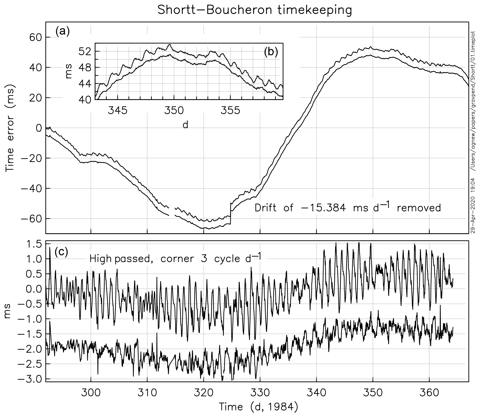
Figure 1Time error of a free pendulum from a Shortt clock, driven by an optical, electronic and mechanical system designed by Pierre Boucheron. A steady rate of s d−1 has been removed. Inset (b) in (a) shows part of the record in more detail, and (c) the data are shown after removing low frequencies. In all cases a residual after subtracting the theoretical gravity tide (converted to pendulum frequency and integrated) is shown slightly below the data.
The effect of tides on pendulum clocks appears to have first been examined by Jeffreys (1928), following a suggestion by the amateur horologist Clement O. Bartrum. He also examined the variations in Earth's rate of rotation caused by the long-period tides, something not detectable without better measurements of both time and Earth orientation. Harold Jefferys' response combined the astronomical expressions for the tides with the response of a clock; it is simpler to start with how changes in gravity affect timekeeping and then use the harmonic description of the tides.
With a few (and very imprecise) exceptions, all clocks depend on an oscillator with some frequency f(t), which is converted to phase (e.g., the position of a clock hand on its dial) according to
which in turn is converted to time by the assumed frequency of the oscillator f0 to give a measured time Tm:
so that if f(t)=f0, Tm is the true time T. If, however, there is a frequency error , there will be a corresponding error in phase ϕ, which in horological terms means a time error:
Clock performance can thus be described in terms of fractional-frequency error fe(t)∕f0, known in horology as the rate and usually expressed in seconds per day. For pendulum clocks it is difficult to measure this with high accuracy, and in all the cases described here the actual measurement was of Te(t), given by Eq. (1), from which an average of fe(t)∕f0 can be found for some interval of observation.
The frequency of a pendulum is given, for small arcs of swing, by
where g is the gravitational acceleration, l the length of the equivalent simple pendulum (with all mass at a point) and 2θ is the total arc of swing (Baker and Blackburn, 2005). Typically θ is less than 1∘, or 0.02 rad, so the term in θ2 may be disregarded for finding the derivative needed. This is the partial derivative of fe∕f0,
so that , where gc(t) is the time-variable part of gravity and g is its average value.
A sense of the tidal effects is best gotten by using a harmonic expansion of the tide and looking at individual harmonics. This can be done using Eqs. (7), (8), (11) and (18) of Agnew (2015); note that Eq. (18) is missing a factor of 2. The fractional change in pendulum frequency from a tidal harmonic of amplitude A, frequency ζ and phase α is
where n and m are the degree and order of the tide; for the tides considered here, n=2. The other variables are ae (Earth's equatorial radius), ge (gravitational acceleration there), g (local gravitational acceleration), δn (gravimetric factor), (normalization coefficient) and (associated Legendre polynomial). The location is given by the colatitude φ and longitude λ. For n=2 the gravimetric factor is given by , where h2 and k2 are the Love numbers for vertical displacement and potential change. For the Preliminary Reference Earth Model, δ2=1.1562.
Taking the integral of Eq. (4) gives, for the time-independent amplitude,
Letting g=ge for simplicity, Table 1 gives the resulting values for the largest tidal harmonics (all those with amplitudes more than 10−4 s). The largest harmonic by far is that associated with the nodal tide (period of 18.6 years). All of the diurnal and semidiurnal tides have amplitudes less than a millisecond.
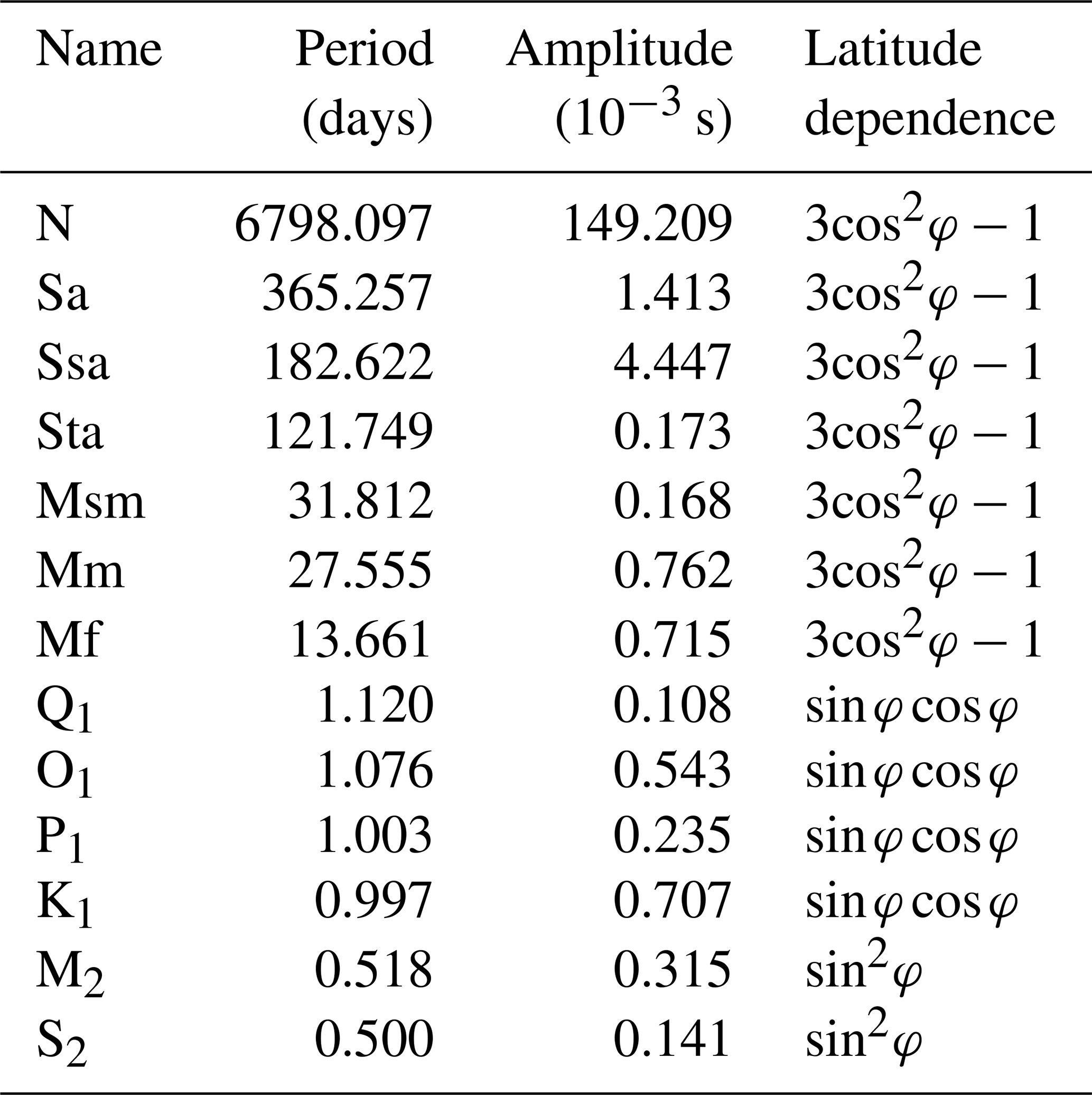
Jeffreys (1928) obtained similar results; perhaps because of a mistake in normalization, the final amplitudes he gave for the tidal harmonics of Te are about 1.4 times those in Table 1. He stated that while the long-period effects are the largest, their detection would require a level of long-term stability not seen in pendulum clocks and described the shorter-term changes as “within the limits of error of the most accurate time-measurements, but perhaps not so far within them as to be entirely devoid of interest”.
One further point can be made about tidal measurements with pendula. Equation (3) means changes in g can be inferred from changes in f directly: the scale factor from fractional frequency to gravity is just 2g, which can easily be determined to a precision and accuracy of 10−4. Since the pendulum is a kind of falling-weight measurement, it is not surprising that it provides a measure of changes in g that can be tied back to standards of length and time. This is not at all the case with spring gravimeters, the calibration of which was difficult until portable and highly precise free-fall absolute gravimeters were developed. It is now routine to use absolute gravimeters to check the drift and scale factor of spring gravimeters intended for tidal measurements (Hinderer et al., 2007). But a pendulum that can record the tides needs no calibration.
As noted above, it is not possible to measure the effects of gravity tides on pendulum clocks without another clock that is not affected by gravity. No such clock of adequate accuracy existed until the 1920s, when electronically maintained oscillators such as tuning forks and quartz crystals were developed. The first quartz-crystal clock was developed by Warren Marrison in 1927 (Katzir, 2016); very soon after (1929) it was used for the study of pendulum clocks. This project was initiated (and funded) by Alfred L. Loomis (Conant, 2002), who turned to various scientific investigations after a very successful legal and financial career had brought him great wealth.
Loomis' study of pendulum clocks comprised three elements (Loomis, 1931). The first was an electrical signal maintained at 1000 Hz by the quartz oscillator operated by Marrison at Bell Telephone Laboratory in Manhattan and provided (over a dedicated telephone line) to Loomis' private laboratory, 65 km away in Tuxedo Park (41.1835∘ N, 74.2144∘ W). The second was three of the highest-quality pendulum clocks then available, the Shortt–Synchronome clock (described below). The third was a chronograph developed by Loomis, which used a rotating arm driven by the 1000 Hz signal at 10 revolutions per second, which could cause a spark to burn a hole in a slowly moving paper record whenever a signal was received. The least count of this system (to use the current term) was 10−3 s; signals from the three Shortt–Synchronome clocks were recorded every 30 s, and changes between them or between them and the quartz oscillator could easily be monitored.
Shortt–Synchronome clocks will appear three times in this account, so a brief description of them is appropriate; much more detail is available in Hope-Jones (1940) and Miles (2019), though the most accessible description is given by Woodward (1995). The double name reflects the nature of these clocks, which consisted of a pair of pendulum systems. One was the Synchronome, an electromechanical clock manufactured by the company of that name to serve as a controller of many subsidiary clocks, sending out signals at regular intervals. The other pendulum, designed by engineer William H. Shortt, was the heart of the system: it swung freely in a container evacuated to a pressure of 3 kPa. The only exception to its free motion was that every 30 s, in response to a signal from the Synchronome clock, a pivoted lever was lowered onto a small wheel attached to the Shortt pendulum. As the pendulum swung away from the lever, the lever fell off the wheel, applying a slight horizontal force to the pendulum; in horological terminology, this is called impulsing the pendulum. The lever's fall was arrested by contact with a switch which performed two actions: it caused the lever to be raised and reset, ready for the next 30 s signal, and it actuated a mechanism to speed up the Synchronome clock if it had fallen behind, which it was deliberately designed to do. So the Shortt free pendulum controlled the overall timekeeping but did so in a way that involved minimal interaction with the Synchronome clock, thus approximating as much as possible a completely free and undamped pendulum – and thanks to the evacuation of the pendulum chamber, the Q factor of the free pendulum was approximately 105.
Loomis supported not just the measurements but also the associated data analysis, conducted by Ernest W. Brown (developer of lunar theory) and his student Dirk Brouwer (Brown and Brouwer, 1931), with, as was usual in those days, “a large amount of calculation, most of which was performed by Mrs. D. Brouwer.” Of the various results, the one of interest for this paper was the effort to look for a lunar effect in the difference between the pendulum and quartz timekeeping. This was done by using a form of stacking of the data (Brown, 1915). The values were taken at hourly intervals and each was assigned to the nearest “lunar hour”: that is, 0.04167 of the lunar day of 24.83 h. All values for a particular lunar hour were summed and averaged. This procedure, viewed as a digital filter, has a response close to one at multiples of the M1 tidal frequency of 0.9664463 cycles d−1 and so should mostly show the effect of the M2 tide.
Figure 2 shows the results plotted in Fig. 3 of Brown and Brouwer (1931), specifically the result of an analysis of 147 d of data of the difference between one of the Shortt clocks (since it was denoted as “Clock 1”, it was probably serial number 20) and the quartz frequency standard. As would be expected, a similar analysis of the three pendulum clocks relative to each other did not show any clear variation. Fitting sinusoids with frequencies of 1 and 2 cycles per lunar day removes all of the variation; the diurnal sinusoid has an amplitude of s with a phase of 178∘; the semidiurnal sinusoid has an amplitude of s with a phase of 166∘.
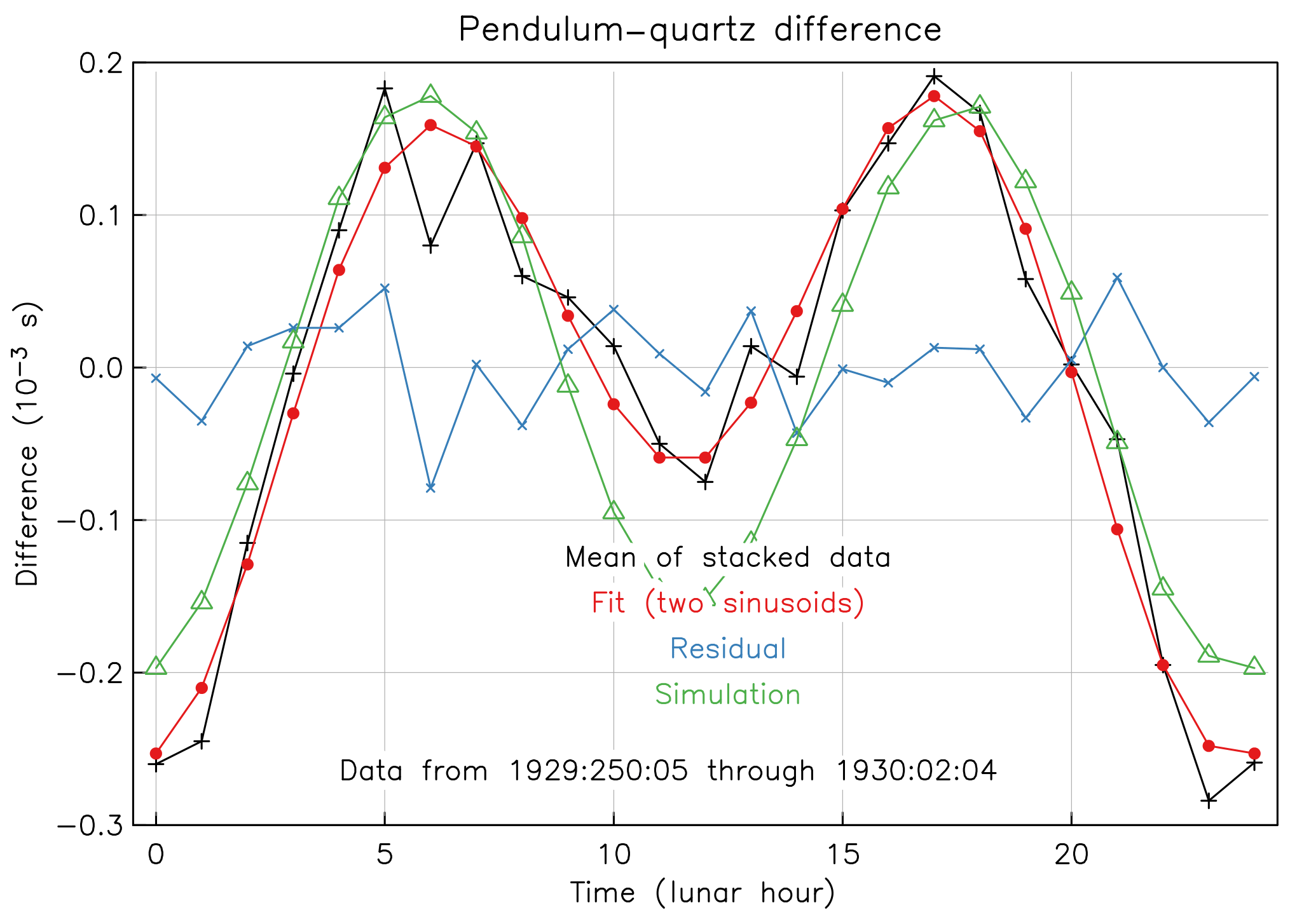
Figure 2Analysis and simulation of a 147 d record of relative time between a Shortt–Synchronome clock and a quartz frequency reference. The black line with pluses shows the stacked results from Brown and Brouwer (1931); the red line with filled circles shows a least-squares fit to this of two sinusoids; the blue line with crosses shows the residual from that fit; and the green line with triangles shows the results of a similar analysis of the theoretical tide for this location and time period. Please note that the date format used in the figure is year:day of year:solar hour.
Brown and Brouwer (1931) noted that the variation was approximately that expected on a rigid Earth, something they found puzzling because of their mistaken idea that gravity variations on an elastic Earth would be times the rigid-Earth variations. They attempted to explain their observation by a large ocean-loading effect but seem to have decided that their results were inconclusive.
In order to re-evaluate their results, I produced a simulation of the tidal time changes at this location and time, using the “SPOTL” (Some Programs for Ocean-Tide Loading) package (Agnew, 2012); ocean loading was computed from the TPXO7.2 global model and the OSU (Oregon State University) local model for eastern North America, though this loading turns out to alter the predicted time by less than 5 %. Figure 2 also shows the result of an analysis of this predicted tide done by averaging values assigned to the same lunar hour. The two series appear similar; again fitting two sinusoids, the diurnal sinusoid has an amplitude of s with a phase of −161∘ not in agreement with the fit to the data. But the semidiurnal sinusoid has an amplitude of s with a phase of 170∘, which is to say 10 % larger and almost exactly in phase with the analyzed data. Given the quality of the measurements, this is excellent agreement.
So these pendulum clocks were able to detect and accurately measure tidal changes in the amplitude of gravitational acceleration g. At this time almost all Earth tide measurements were of tilt, which is to say changes in the direction of gravity. Lambert (1931) does not mention any observations of tidal changes in g, while Lambert (1940) describes only some measurements made in the US in 1938–1939. The first successful observation of tidal changes in g that I have found is that by Tomaschek and Schaffernicht (1932), who showed a few days of data and analyzed 2 months worth, but they would appear to have had a calibration problem, since their result for δ was 0.64, 55 % of the true value. As noted in Sect. 2, pendulum measurements are free from calibration uncertainties.
The next attempt to measure tidal effects with pendulum clocks was by Stoyko (1949) and explicitly aimed at using tidal gravity to determine δ, which when combined with tidal tilt measurements could provide values for the two Love numbers h and k. The measurements were made at the Paris Observatory (48.8364∘ N, 2.3365∘ E), a good choice in two ways. First of all, it was the location of the Bureau Internationale de l'Heure (BIH), the entity responsible for defining a unified time system by determining corrections (after the fact) to the time signals broadcast by different countries and based on timekeeping from different observatories. Broadcast time signals showed unexpectedly large deviations between different timekeepers, and the BIH was established to deal with this (Kershaw, 2019). Given this mandate, the BIH maintained a relatively large ensemble of clocks. These were housed in a vault at 23 m depth, much deeper than most other timekeepers, a setting where even annual variations in temperature would be small and ground noise would be attenuated.
In looking for tides, six of the BIH clocks were used. One was a Shortt–Synchronome clock (number 44), while four were precision pendulum clocks built by the French firm of Leroy et Cie (Roberts, 2004). These were as simple as the Shortt–Synchronome clock was complex: a single pendulum driven by an escapement that used springs to provide a nearly invariant impulse to the pendulum (Martin, 2003), only two wheels in the gear train and a gravity drive using a 7 g weight electrically rewound every 30 s. As in the Shortt–Synchronome clock, the pendulum operated inside a sealed tank, though at a pressure (80 kPa) not far below atmospheric. The sixth timekeeper was a tuning-fork frequency standard built by the electronics firm of Belin.
The differences between these timekeepers was recorded twice daily, at 08:10:30 and 20:10:30 universal time, on a high-speed chronograph, recording on paper at 0.25 m s−1. These 12 h samples were then (in today's terms) convolved with a high-pass filter with weights (1, −3, 3, −1) (removing any constant, linear or quadratic behavior) and then, it appears, analyzed as daily samples. The Nyquist frequency was thus reduced to 0.5 cycles d−1, so the M2 tide would have been aliased to a period of 14.7 d, while the K1 and P1 harmonics would both have been aliased to a frequency of 1 cycle per year. Monthly means were created, with an annual variation fit to them to determine the size of these diurnal tides. For the M2 tide each difference was assigned to the nearest lunar hour, and a year of these was summed. Comparison with equivalently processed rigid-Earth tides then allowed the gravimetric factor δ to be found for each year from 1940 through 1943.
Figure 3 shows the values of δ (normalized against what we now know is the true value) determined for the five clocks over 4 years for both the K1 − P1 and M2 tides. While there is a great deal of scatter, the median value of the normalized δ is 1.05. It is notable that the scatter of the estimates increases for the last 2 years compared to the first 2 years: given that Paris was under German occupation, it can easily be imagined that replacement parts for delicate instruments of this kind might have been difficult to get. But these results, at the time they were published, were not drastically worse than what had been attained by gravimeter measurements. It does not appear that the Leroy clocks were significantly worse at measuring tides than the Shortt–Synchronome clock, though it is likely that the extremely stable environment they were operated in played a part in allowing this.
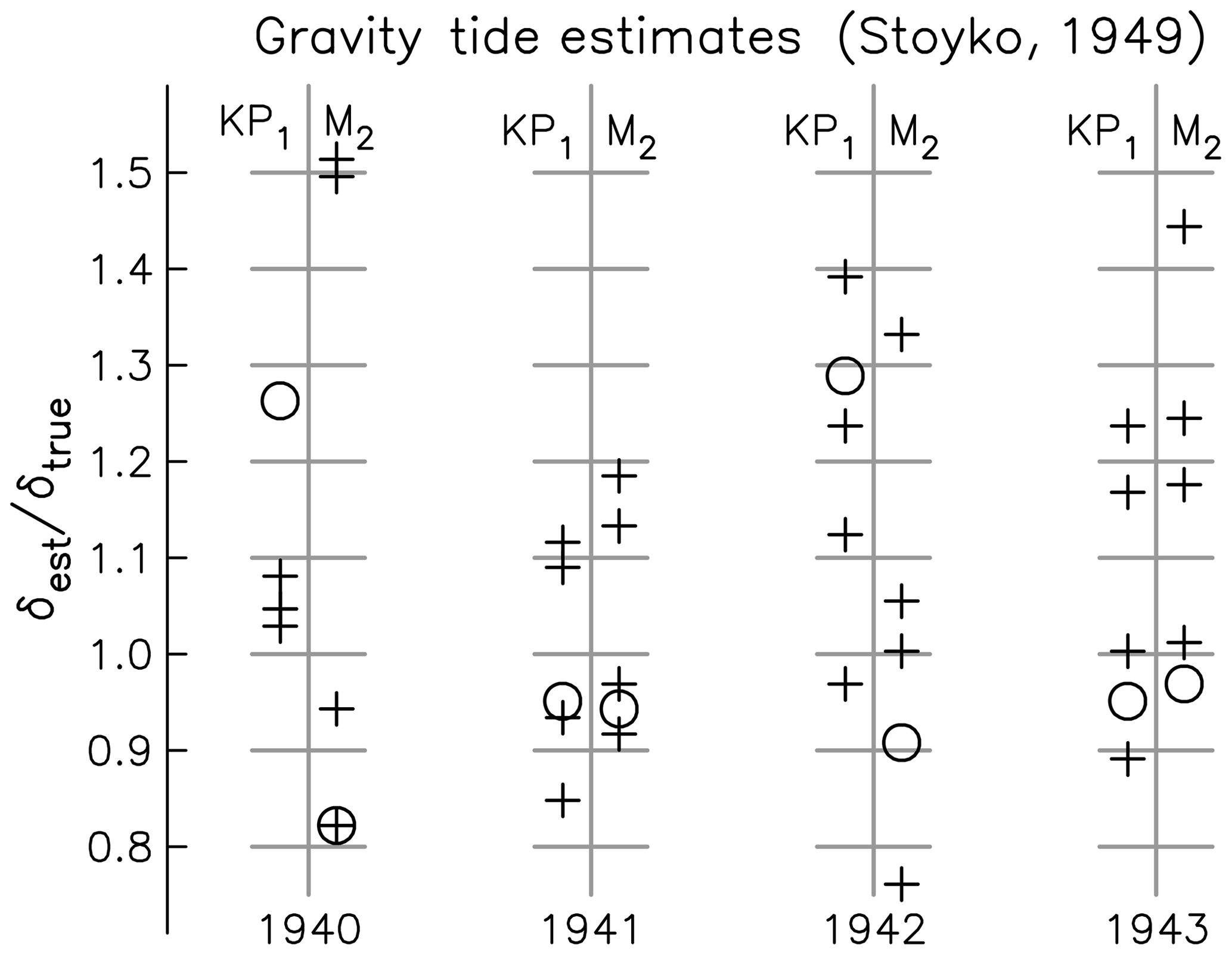
Figure 3Results for the tidal gravimetric factor obtained by different clocks and analyses in Paris between 1940 and 1943. The circles indicate the results from the Shortt–Synchronome clock, and the pluses show the results from the Leroy clocks.
While quartz clocks became the best measurers of time in the 1940s, pendulum clocks remained popular in some settings, since they did not require specialized electronics expertise to maintain. Judging by the sales of the Shortt–Synchronome clocks, this was particularly the case in Communist countries: of the 31 such clocks sold after 1945 (Miles, 2019), 19 went to the People's Republic of China, eastern Europe or the Soviet Union (USSR). Indeed, the USSR built its own version of the Shortt–Synchronome clock, the “Etalon” clocks (Roberts, 2004). And in addition, the USSR introduced and manufactured an alternate design of pendulum clock, one very different from the Shortt–Synchronome clock.
These clocks were invented by Feodosii Mikhailovich Fedchenko; Feinstein (2004) is the fullest English-language description. Three models were produced, the AchF-1, AchF-2 and AchF-3, all of which used a pendulum suspension that removed the θ2 term in the frequency expression given in Eq. (2). This term exists because the restoring force on a pendulum varies as sin θ rather than θ, creating a slightly nonlinear system in which the frequency depends on the amplitude of swing. From Eq. (2), the dependence of a normalized frequency on the angle of swing is
which, for a typical arc of swing of rad, is . So a variation of fractional frequency of 10−8 would be produced by a fractional change in arc of approximately .
For small arcs, the change in height of the bob is proportional to the square of the arc, so the arc is approximately proportional to the square root of the energy of the pendulum. In a steady state, this energy is proportional to the energy input, so a frequency change of 10−8 would be created by a fractional change in energy input of , a stability that is difficult to achieve. Fedchenko's accomplishment was to devise a method for eliminating the θ2 term in Eq. (2), making the pendulum what is termed isochronous. He accomplished this by suspending the pendulum from three steel strips, with one longer than the other two; this created an additional elastic restoring force that could be adjusted to cancel the θ2 term (Woodward, 1999). While there had been earlier proposals for elastic devices to make a pendulum isochronous (Phillips, 1891, 1892; Bush and Jackson, 1951), Fedchenko's seems to have been the only one to see actual use.
The pendulum of the AchF-3 swung in a low vacuum (0.4 kPa); its position was sensed, and a force was applied to it electromagnetically. Permanent magnets were mounted on the pendulum and passed through a pair of coils at the bottom of its arc. These coils were fixed to a rod that would expand and contract with temperature in parallel with the pendulum, keeping the geometry of the magnet-coil system unchanged. As the magnets moved past the coils, they generated a voltage in one coil, and on alternate swings this voltage was applied to a two-stage transistor amplifier that produced a current in the second coil in the opposite sense to that induced in the first, applying a small force to the pendulum. The amplifier in this feedback system was driven by a small constant-voltage battery: the power consumption was about 60 µW.
The best evidence for the detection of tidal fluctuations of this clock comes from Agaletskii et al. (1970); the senior author was a metrologist with an interest in absolute measurements of g (Cook, 1965), who wished to present the clock as a direct measurement of the tidal fluctuations that would affect any determination of g. The data were collected at the All-Union Scientific Research Institute for Physical-Engineering and Radiotechnical Metrology in Mendeleyevo, outside of Moscow (56.038∘ N, 37.232∘ E). A total of 6 months of records were shown for September through December of 1968 and 1969. The data curves are clearly hand-drawn. Agaletskii et al. (1970) state that it was not until after 6 months of “hunting” by the feedback mechanism that the rate became steady; this was probably because of the high Q of the pendulum, probably several times 105 (Bateman, 1977).
Figure 4 shows the data from the clock: the tides are clearly visible. I again computed the theoretical tide for this location using SPOTL and shifted the time of observations by subtracting 3 h to go from Moscow to Universal Time. Subtracting this from the data produces a series with a noticeably lower variance. Shifting the times further (1.25 more hours for the 1968 data and 1.75 more hours for the 1969 data) produces the lowest variance and the least amount of visible tidal signal in the residual: this is an acceptable adjustment, given the crudeness in digitizing a hand-drawn curve. Allowing for a scale factor between the theoretical tides and the observations produces a factor of 0.9 for both years. Clearly the clock data measure the diurnal and semidiurnal tides. Alexeev and Kolosnitsyn (1994) used these data and a longer set of daily data to show that the Mf tide could also be detected.
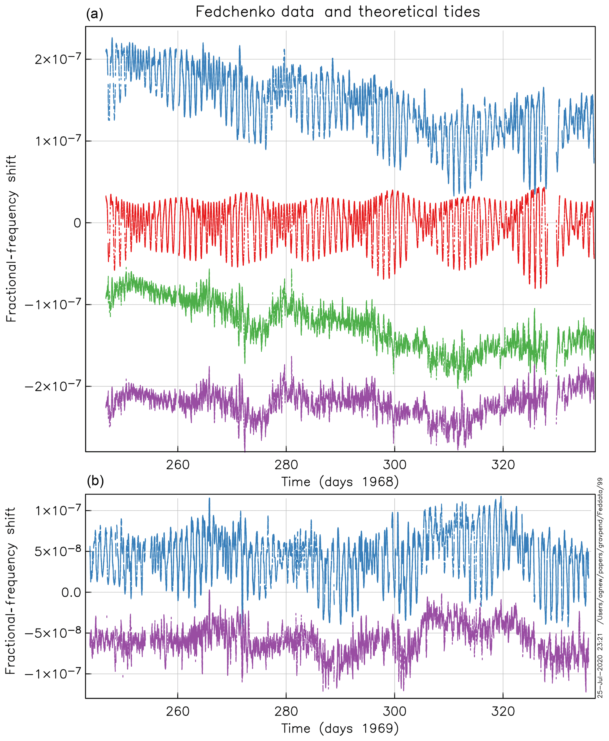
Figure 4Rates of the Fedchenko clock over a 3-month period in 1968 (a) and 1969 (b). Rates were determined by time differences with an atomic clock over 2 h intervals and hand-plotted. In (a) the uppermost trace is the point cloud produced by an image-processing digitization of the plotted data; scales were determined against tic marks in the original plot. The trace below is the theoretical tide at the times of each point, and the one below that is the residual from subtracting them. The bottom trace is the residual when the theoretical tides are fit to the observed, allowing for a scaling factor. Panel (b), for 1969, shows only the original data and the residual.
The final measurement discussed here returns to the Shortt–Synchronome clock, only without the Synchronome. In 1932, Shortt–Synchronome serial number 41 was installed in the U.S. Naval Observatory (USNO; 38.922∘ N, 77.067∘ W) as a sidereal time standard: that is, a clock that could be directly compared with astronomical observations. By 1946, all pendulum clocks at USNO had been replaced by quartz-crystal clocks (Sollenberger and Mikesell, 1945) but were left in the specially built clock vault (Dick, 2003). Almost 40 years later, Pierre Boucheron, an engineer and amateur horologist, visited USNO to look for information on their clocks' performance. While there, he visited the clock vault and found that the original Shortt pendulum for number 41 was there and still under vacuum; he also found that a mirror had been attached to the pendulum and an optical-flat window had been installed in the bell jar that was the top part of the vacuum enclosure. With USNO's permission, he set up an optical lever to measure the pendulum's motion, sending current from a photocell to some simple logic circuits that, every 30 s, dropped the impulsing lever just as the Synchronome had. A second photocell sent timing pulses to a counter which was read every hour and compared with the USNO atomic master clock (Boucheron, 1985). Boucheron called this system, like the Synchronome part of the Shortt–Synchronome clock, a “slave” system; but unlike the Synchronome, it did not have any timekeeping ability, and the position of the Shortt pendulum was used directly to release the impulse lever. As Boucheron pointed out, the optical-sensing system probably had less variability in sensing the time of swing than the electromechanical switches and contacts of the Shortt–Synchronome clock.
This system operated for just under a year, from 1984:292 (year:day of year) through 1985:278. Boucheron (1986, 1987) described the clock's performance. As a timekeeper it was poorer than might be expected, showing variations of up to 1.5 s over the course of the year. But the clock's short-term stability was good enough that Earth tides were visible in plots of the hourly rate. Boucheron (1987) discussed the tidal response in more detail, although his analysis did not go much beyond that of Brown and Brouwer (1931).
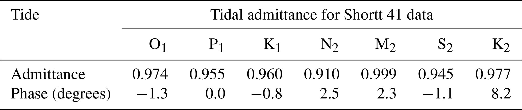
These data were transcribed by Philip Woodward in order to perform a spectral analysis (Woodward, 1995); in keeping with earlier results (and standard horological practice) he differenced the times to produce hourly rates. Machine-readable hourly rate data are available over the full span of observation; the time differences plotted in Fig. 1 are available only for the first 3 months. Again, to compare rates with the tidal fluctuations I computed the theoretical gravity tide using SPOTL; here too the ocean load tide does not have a large effect. Parallel harmonic analyses of the gravity signal and the hourly rates give, for the major tides, the complex value of the ratio of observed to theoretical tides (the admittance).
Table 2 gives the results for the larger tidal harmonics. Except for M2, all the admittance amplitudes are a few percent below one, with phase differences scattered about zero. A 2∘ phase shift is the same magnitude as a 4 % change in amplitude, so it is reasonable to believe that this scatter comes from background noise at the tidal frequencies.
Table 2Ratio of observed to model tides. The admittance amplitude is relative to the theoretical value of tidal change in pendulum frequency, assuming local gravity to be 9.8008 m2 s−1; the admittance phase is the difference in degrees, with lags being negative.
To determine this noise level I computed the power spectral density of the rate data in two ways. First, I computed the periodogram of the data: that is, computing the discrete Fourier transform and finding the amplitude at each frequency. While this estimate of the PSD (power spectral density) can be biased and is always inconsistent (in the statistical sense), it is the best way to show narrowband signals such as the tide.
Fitting tidal harmonics to the data leaves no tidal lines visible in the periodogram, which means that more averaging of the spectral estimates is appropriate. The second set of spectrum estimates were found using the adaptive multitaper method described by Barbour and Parker (2013). This minimizes a combination of the local bias caused by curvature of the power spectrum and the uncertainty of the estimates. The relative weighting of these two components of spectral error is adjustable, and Fig. 5 shows the spectrum for three different values of the parameter. As less weight is given to minimizing local bias, the spectrum becomes less smooth; in this case the main effect is to reduce bias at the very lowest frequencies.
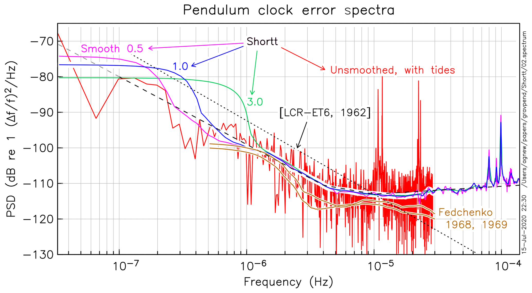
Figure 5Power spectra of fractional-frequency changes in the Shortt clock as modified by Boucheron and the Fedchenko clock. For the Shortt clock, the spectrum is computed for a periodogram (red); this includes tides but is not shown for all frequencies. The blue, green and purple lines are estimates for the same spectrum done using an adaptive spectrum estimation method, for different values of the relative weighting of local bias and spectral stability. The black dashed line is an “eyeball fit” to the spectrum, plotted in gray when it is extrapolated. The spectra for the two 3-month spans of detided Fedchenko data (Fig. 4) are shown in brown. The black dotted line represents the noise level of a LaCoste & Romberg Earth tide gravimeter (Slichter et al., 1964), from data collected in 1961–1963 (LCR-ET6). See the text for additional information.
Along with the tides, the spectra show several peaks at periods around 2.8 to 3.5 h, which are clearest in the multitaper estimate. These periods are much longer than the period of the gravest normal mode, which itself is far too small to be visible in these data. The source of these spectral peaks is not understood but is assumed to be some irregularity in the mechanical system that drives the pendulum. Loomis (1931) noted that each of his clocks showed a characteristic pattern of short-term variations.
The noise level of the Shortt–Boucheron clock can be described by a PSD which varies as a power of frequency fβ over three different frequency bands. For frequencies less than Hz (periods longer than 70 h), the exponent of the power law is : essentially the same random-walk behavior found by Woodward using the Allan variance (see chap. 18 of Rawlings, 1993) and (though not identified as such) by Greaves and Symms (1943). This behavior is undesirable because it diverges with time, and its integral, the time error (what clocks are supposed to measure), diverges even more rapidly. For periods from 70 to 28 h, , which is close to flicker noise; for periods less than 28 h, β=0.2, which is close to white noise, though clearly increasing with frequency. It is quite possible that this increase (and the mystery peaks) comes from variations at even shorter periods that appear to be at longer ones because of the hourly sampling.
Figure 5 also shows the PSD of the two residual series of the Fedchenko data, plotted in Fig. 4. To obtain the equispaced data needed for these spectra, a local regression (loess) was done on the point cloud, and the results linearly interpolated to a 0.05 d interval, which is comparable to the original 2 h spacing. I estimated the PSD using the same adaptive method; given that the series was derived from hand-plotted data, the true PSD is very likely below the ones shown. It is clear that the Fedchenko clock, in this frequency band, is definitely less noisy than the Shortt–Boucheron system.
Despite the extreme difficulty of making clock pendula respond only to changes in gravity and nothing else, the best pendulum clocks have shown the ability to detect tides, with the first example preceding any gravimeter measurements. And pendulum measurements, like other falling-mass systems, provide a result that is easily calibrated: the result of Brown and Brouwer (1931), properly interpreted, would have given an accurate value of the factor δ for the gravity tides.
The observations reviewed here also make a horological point, namely that there is more than one way for a pendulum clock to have the performance demanded – something recently demonstrated by the excellent performance of a clock deliberately designed to make use of the nonlinear part of Eq. (2) to compensate for environmental changes (McEvoy and Betts, 2020).
The developers of the Shortt clock emphasized that it used a free pendulum, which was only impulsed at longer intervals and in a way that required no input from the pendulum. But neither the Leroy nor the Fedchenko clock had this feature: in both, the pendulum was used to time the impulse, and this impulse was given frequently. It also does not seem to have been necessary for the pendulum to swing in an evacuated space, since the range of vacua in these clocks was from 0.4 to 80 kPa. The Littlemore clock of Hall (2004), built in the 1990s, aimed at improved performance by having an even freer pendulum operating in a high vacuum ( Pa) and being impulsed electromagnetically. Though over 250 d its timing error was within 50 ms, its short-term stability was poor: a spectrum of the rate data, if plotted in Fig. 5, would be a white spectrum at −88 dB.
While the first measurements of gravity tides were better made by clocks than by gravimeters, the latter rapidly improved, partly thanks to the stimulus of military and industrial funding (Warner, 2005). Figure 5 shows a gravimeter noise spectrum from 1962; at tidal frequencies this is comparable to the best clock performance. Modern superconducting gravimeters have a much lower noise level: for fractional gravity change, it is −155 dB for periods of 12 to 24 h, while modern spring gravimeters are only about 6 dB noisier (Rosat et al., 2004, 2015; Calvo et al., 2014).
So “tide from time” is now not at all the best measurement of gravity changes but a signal that can demonstrate good short-term oscillator performance. Horological measurements of gravity span over 3 and a half centuries; even though their utility is now gone, it has been an interesting journey.
The data shown in Figs. 1 and 2 are available from the author. The data shown in Fig. 4 are available from Agnew (2020, https://doi.org/10.5281/zenodo.3978746).
The author declares that there is no conflict of interest.
This article is part of the special issue “Developments in the science and history of tides (OS/ACP/HGSS/NPG/SE inter-journal SI)”. It is not associated with a conference.
I thank Bob Holmström and Tom Van Baak for discussions: more specifically I thank Bob Holmström for alerting me to the 1949 paper by Stoyko (Stoyko, 1949) and the 1994 paper by Alexeev (Alexeev and Kolosnitsyn, 1994) and Tom Van Baak for providing me with the Shortt 41 rate and Littlemore time data and for reminding me about the need to consider time shifts in data fitting. The gravimeter data used for the spectrum in Fig. 5 were provided to Walter Munk by Louis B. Slichter in 1964; their preservation over the next half century is due to the efforts of Florence Oglebay Dormer and David Horwitt. I thank Walter Zürn and another referee for their helpful reviews.
This paper was edited by Mattias Green and reviewed by Walter Zürn and one anonymous referee.
Agaletskii, P. N., Vlasov, B. I., and Fedchenko, F. M.: Experimental determination of variations in the force of gravity with the help of the pendulum clock AChF-3, Proc. All-Union Sci. Res. Inst. Phys-Engin. Radiotech Metrol. (VNIIFTRI), 40, 1–10, 1970. a, b
Agnew, D. C.: SPOTL: Some Programs for Ocean-Tide Loading, Sio technical report, Scripps Institution of Oceanography, available at: http://escholarship.org/uc/item/954322pg (last access: 12 July 2020), 2012. a
Agnew, D. C.: Earth tides, in: Treatise on Geophysics, edited by: Herring, T. A., 2nd Edn., Geodesy, 151–178, Elsevier, New York, 2015. a, b
Agnew, D.: Tidal Gravity Variations Measured by a Fedchenko AChF-3 Precise Pendulum Clock [Data set], Zenodo, https://doi.org/10.5281/zenodo.3978746, 2020. a
Alexeev, A. D. and Kolosnitsyn, N. I.: The pendulum astronomical clock AChF-3 as a gravimeter, Bull. Inf. Marees Terr., 119, 8881–8884, 1994. a, b
Baker, G. L. and Blackburn, J. A.: The Pendulum: A Case Study in Physics, Oxford University Press, Oxford, 2005. a
Barbour, A. J. and Parker, R. L.: PSD: Adaptive, sine multitaper power spectral density estimation for R, Comp. Geosci., 63, 1–8, https://doi.org/10.1016/j.cageo.2013.09.015, 2013. a
Bateman, D. A.: Vibration theory and clocks, Part 3: Q and the practical performance of clocks, Horol. J., 120, 48–55, 1977. a
Boucheron, P. H.: Just how good was the Shortt Clock?, Bull. Nat. Assoc. Watch Clock Collect., 27, 165–173, 1985. a
Boucheron, P. H.: Effects of the gravitational attraction of the Sun and Moon on the period of a pendulum, Antiq. Horol., 16, 53–65, 1986. a
Boucheron, P. H.: Tides of the planet Earth affect pendulum clocks, Bull. Nat. Assoc. Watch Clock Collect., 29, 429–433, 1987. a, b
Brown, E. W.: Simple and inexpensive apparatus for tidal analysis, Am. J. Sci., 39, 386–390, https://doi.org/10.2475/ajs.s4-39.232.386, 1915. a
Brown, E. W. and Brouwer, D.: Analysis of records made on the Loomis chronograph by three Shortt clocks and a crystal oscillator, Mon. Not. R. Astron. Soc., 91, 575–591, https://doi.org/10.1093/mnras/91.5.575, 1931. a, b, c, d, e, f
Bullard, E. C. and Jolly, H. L. P.: Gravity measurements in Great Britain, Geophys. J. Int., 3, 443–477, 1936. a
Bush, V. and Jackson, J. E.: Correction of spherical error of a pendulum, J. Frankl. Inst., 252, 463–467, 1951. a
Calvo, M., Hinderer, J., Rosat, S., Legros, H., Boy, J., Ducarme, B., and Zürn, W.: Time stability of spring and superconducting gravimeters through the analysis of very long gravity records, J. Geodyn., 80, 20–33, https://doi.org/10.1016/j.jog.2014.04.009, 2014. a
Conant, J.: Tuxedo Park: A Wall Street Tycoon and the Secret Palace of Science That Changed the Course of World War II, Simon & Schuster, New York, 2002. a
Cook, A. H.: The absolute determination of the acceleration due to gravity, Metrologia, 1, 84–114, https://doi.org/10.1088/0026-1394/1/3/003, 1965. a, b
Dick, S. J.: Sky and Ocean Joined: the U.S. Naval Observatory, 1830–2000, Cambridge University Press, New York, 2003. a
Feinstein, G.: F. M. Fedchenko and his precision astronomical clocks, in: Precision Pendulum Clocks: France, Germany, America, and Recent Advancements, edited by: Roberts, D., 247–263, Schiffer Publishing, Atglen, PA, 2004. a
Graham, G. and Campbell, C.: An account of some observations made in London and at Black-River in Jamaica, concerning the going of a Clock; in order to determine the difference between the lengths of isochronal pendulums in those places, Philos. T. R. Soc. Lond., 38, 302–314, https://doi.org/10.1098/rstl.1733.0048, 1733. a
Greaves, W. M. H. and Symms, S. T.: The short-period erratics of free pendulum and quartz clocks, Mon. Not. R. Astron. Soc., 103, 196–209, 1943. a
Hall, E. T.: The Littlemore clock, in: Precision Pendulum Clocks: France, Germany, America, and Recent Advancements, edited by: Roberts, D., 264–273, Schiffer Publishing, Atglen, PA, 2004. a
Hinderer, J., Crossley, D., and Warburton, R.: Gravimetric methods: superconducting gravity meters, in: Treatise on Geophysics: Geodesy, edited by: Herring, T. A., 65–122, Elsevier, New York, 2007. a
Hope-Jones, F.: Electrical Timekeeping, N.A.G. Press, London, 1940. a
Jeffreys, H.: Possible tidal effects on accurate time-keeping, Geophys. Suppl. Mon. Not. R. Astron. Soc., 2, 56–58, 1928. a, b
Kater, H.: An Account of experiments for determining the length of the pendulum vibrating seconds in the latitude of London, Philos. T. R. Soc. Lond., 108, 33–102, https://doi.org/10.1098/rstl.1818.0006, 1818. a
Kater, H.: An account of experiments for determining the variation in the length of the pendulum vibrating seconds, at the principal stations of the Trigonometrical Survey of Great Britian, Philos. T. R. Soc. Lond., 109, 337–508, https://doi.org/10.1098/rstl.1819.0024, 1819. a
Katzir, S.: Pursuing frequency standards and control: the invention of quartz clock technologies, Ann. Sci., 73, 1–39, https://doi.org/10.1080/00033790.2015.1008044, 2016. a
Kershaw, M.: Twentieth-Century longitude: When Greenwich moved, J. Hist. Astron., 50, 221–248, https://doi.org/10.1177/0021828619848180, 2019. a
Lambert, W. D.: Earth tides, Bull. Nat. Res. Council, 78, 68–80, 1931. a
Lambert, W. D.: Report on Earth tides, U.S. Coast and Geodetic Survey Special Publication, 223, 1–24, 1940. a
Lenzen, V. F. and Multhauf, R.: Development of gravity pendulums in the 19th century, U.S. National Museum Bull.: Contributions from Museum History and Technology, 240, 301–347, 1965. a
Loomis, A. L.: The precise measurement of time, Mon. Not. R. Astron. Soc., 91, 569–575, https://doi.org/10.1093/mnras/91.5.569, 1931. a, b
Martin, J.: Escapements, in: Precision Pendulum Clocks: The Quest for Accurate Timekeeping, edited by: Roberts, D., 111–139, Schiffer Publishing, Atglen, PA, 2003. a
Mason, C. and Dixon, J.: Astronomical observations, made in the forks of the River Brandiwine in Pennsylvania, for determining the going of a clock sent thither by the Royal Society, in order to find the difference of gravity between the Royal Observatory at Greenwich, and the place where the clock was set up in Pennsylvania, Philos. T. R. Soc. Lond., 58, 329–335, https://doi.org/10.1098/rstl.1768.0043, 1768. a
Matthys, R. J.: Accurate Clock Pendulums, Oxford University Press, Oxford, 2004. a
McEvoy, R. and Betts, J. (Eds.): Harrison Decoded: Towards A Perfect Pendulum Clock, Oxford University Press, Oxford, 2020. a
Miles, R. A. K.: Synchronome: Masters of Electrical Timekeeping, Antiquarian Horological Society, London, 2019. a, b
Olmsted, J. W.: The scientific expedition of Jean Richer to Cayenne (1672–1673), Isis, 34, 117–128, https://doi.org/10.1086/347762, 1942. a
Phillips, E.: Pendule isochrone, CR Hebd. Acad. Sci., 112, 177–183, 1891. a
Phillips, E.: Disposition propre a rendre le pendule isochrone, J. Ecole Polytech., 62, 1–35, 1892. a
Phipps, C. J.: A Voyage Towards the North Pole Undertaken by His Majesty's Command, 1773, J. Nourse, London, 1774. a
Rawlings, A. L.: The Science of Clocks and Watches, British Horological Institute, London, 1993. a
Roberts, D.: Precision Pendulum Clocks: France, Germany, America, and Recent Advancements, Schiffer Publishing, Atglen, PA, 2004. a, b
Rosat, S., Hinderer, J., Crossley, D., and Boy, J. P.: Performance of superconducting gravimeters from long-period seismology to tides, J. Geodyn., 38, 461–476, 2004. a
Rosat, S., Calvo, M., Hinderer, J., Riccardi, U., Arnoso, J., and Zürn, W.: Comparison of the performances of different spring and superconducting gravimeters and STS-2 seismometer at the Gravimetric Observatory of Strasbourg, France, Stud. Geophys. Geod., 59, 58–82, https://doi.org/10.1007/s11200-014-0830-5, 2015. a
Sabine, E.: An account of experiments to determine the acceleration of the pendulum in different latitudes, Philos. T. R. Soc. Lond., 111, 163–190, https://doi.org/10.1098/rstl.1821.0015, 1821. a
Slichter, L. B., MacDonald, G. J. F., Caputo, M., and Hager, C. L.: Report of earth tides results and of other gravity observations at UCLA, Observatoire Royal Belgique Comm. Ser. Geophys., 236, 124–130, 1964. a
Sollenberger, P. and Mikesell, A. H.: Quartz crystal astronomical clocks, Astron. J., 51, 123–124, https://doi.org/10.1086/105851, 1945. a
Stoyko, N.: L'Attraction Luni-Solaire et les pendules, Bull. Astron., 14, 1–36, 1949. a, b
Tomaschek, R. and Schaffernicht, W.: Tidal oscillations of gravity, Nature, 130, 165–166, https://doi.org/10.1038/130165b0, 1932. a
Warner, D. J.: A matter of gravity: Military support for gravimetry during the Cold War, in: Instrumental in War: Science, Research, and Instruments between Knowledge and the World, edited by: Walton, S. A., 339–362, Brill, Leiden, 2005. a
Woodward, P.: My Own Right Time: An Exploration of Clockwork Design, Oxford University Press, New York, 1995. a, b, c
Woodward, P.: Fedchenko's isochronous pendulum, Horol. J., 141, 82–84, 122–124, 1999. a
Yoder, J. G.: Unrolling Time: Christiaan Huygens and the Mathematization of Nature, Cambridge University Press, Cambridge, 1989. a
- Abstract
- Introduction
- The first theoretical treatment, 1928
- A first detection in 1929: Shortt–Synchronome clock
- Collective measurements 1940–1943: an ensemble of clocks
- Improved measurements in the 1960s: Fedchenko
- Digital data in 1984: Shortt–Boucheron
- Conclusions
- Data availability
- Competing interests
- Special issue statement
- Acknowledgements
- Review statement
- References