the Creative Commons Attribution 4.0 License.
the Creative Commons Attribution 4.0 License.
 | 21 Feb 2023
A pioneering time of discoveries in large-scale tropical meteorology: 1960 through 1972
Roland A. Madden
The Australian Bureau of Meteorology (http://www.bom.gov.au/climate/mjo, last access: 9 February 2023) states that “The Madden–Julian Oscillation (MJO) is a major fluctuation in tropical weather on weekly to monthly timescale. The MJO can be characterized as an eastward moving `pulse' of cloud and rainfall near the Equator that typically recurs every 30 to 60 days.” Early descriptions of the MJO were contained in two papers by Madden and Julian (1971, 1972). This paper relates the story of developments in tropical meteorology in the 1960s that led to those two papers. The decade saw the first unambiguous identification of large-scale, theoretically predicted, tropical waves. Spectral analysis was used effectively by researchers to link observations with the theoretically expected features of these waves. At the same time, longer time series of observations, faster computers, and an algorithm designed to speed up Fourier transforms, vital for spectral analysis, all became available. These developments set the stage for the oscillation to be recognized.
- Article
(1444 KB) - Full-text XML
- BibTeX
- EndNote


Clarence Palmer, in his treatise on tropical meteorology, stated that whenever we obtain more data from the tropics, “the results usually astonish us” (Palmer, 1952). That certainly applied to the decade of the 1960s. Tropical data were becoming more accessible in a digitized form suitable for treatment by computers that were also becoming available to meteorologists. Proceeding logically from Clarence Palmer's observation, the stage was set for us to be astonished, and astonished we were.
The decade opened with the discovery of the quasi-biennial oscillation (QBO) in the equatorial stratosphere. It is a most amazing phenomenon. The QBO is remarkable in its approximate 26-month period, in its regular downward propagation, and in its large amplitude. By the mid-1960s, efforts to explain the QBO led to two of the earliest unambiguous identifications of large-scale atmospheric waves predicted by theory. Simultaneously, a theory tailored just for tropical regions was published. Spectral analysis, a particularly powerful analysis tool for the tropics that sometimes requires relating events at stations thousands of kilometers apart, was beginning to be used effectively by researchers. Also, in 1965, a fast Fourier transform algorithm suitable for coding was published that made spectral calculations orders of magnitude faster than traditional ones.
Toward the end of the decade in early 1967, a large-scale field program in the equatorial central Pacific was organized and carried out by the National Center for Atmospheric Research (NCAR; Zipser, 1970; see Fig. 1). Work on data from this field program, the Line Islands Experiment (LIE), introduced me, a rookie researcher at NCAR, to the developments described above. In the fall of 1967, during my first days at NCAR, I sat in the temporarily vacant office of an NCAR scientist, who was spending a sabbatical year at the University of Chicago, from where, coincidently, I had just left – fresh with a master's degree. That scientist was Paul Julian. We were both now members of NCAR's Synoptic Meteorology Group and later the Empirical Studies Group (Fig. 2).

Figure 1National Center for Atmospheric Research, Boulder, Colorado USA (© UCAR).
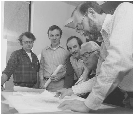
Figure 2Members of the Empirical Studies Group, with (left to right) Paul Julian, Roland Madden, Dennis Shea, Chester Newton (group head), and Harry van Loon, in about 1980 (© UCAR).
Paul Julian was a former student of Hans Panofsky, who pioneered the use of spectral analysis in meteorology (Panofsky, 1955). As a result, Paul Julian was well versed in the technique. He published a review of it and showed how spectral analysis could be applied to geophysical data (Julian, 1967). He had also done a spectral analysis of 21 years of zonal index data (a measure of the strength of the westerlies) to quantitatively test the notion of an index cycle of 3 to 8 weeks (Julian, 1966) that had been qualitatively accepted as real (e.g., Petterssen, 1956). Results suggested that the zonal index could be adequately modeled by a first-order autoregressive process, with little evidence, of a preferred 3- to 8-week variation.
Upon Paul Julian's return to NCAR in 1968, he guided me in my efforts to apply spectral analysis to the LIE winds. By late 1970, our collaboration had expanded and eventually led to a description of what is now referred to as the MJO, or Madden and Julian Oscillation, after two papers in the early 1970s (Madden and Julian, 1971, 1972; hereafter MJ71 and MJ72). What follows is the story, as I remember it, of our collaboration that led to those two papers and of the background outlined above that influenced us.
2.1 Discovery of the quasi-biennial oscillation
Graystone (1959) presented a time–height diagram of zonal, or u wind, in the stratosphere over Christmas Island (2∘ N, 158∘ W). He had only 2 years of data and could not recognize the amazing QBO which he was sampling. He only remarked that there was an absence of an annual cycle and a presence of large vertical shears. Ebdon (1961) and Reed et al. (1961) extended the record beyond 2 years, and they were able to identify east and west wind regimes propagating downward in the stratosphere that varied by as much as 40 m s−1. The average timescale of the wind shifts was 26 months. I am sure that Clarence Palmer, who left us in 1973, was astonished, along with most meteorologists, by the amazing behavior of the QBO. The QBO increased interest in tropical meteorology. Although the QBO did not affect our later work directly, some subsequent research aimed at explaining its behavior did.
2.2 Theory of waves in the equatorial atmosphere
Matsuno (1966) published a theoretical paper specifically tailored to the equatorial region. He showed how his approximate equations are an asymptotic case of the Laplace tidal equations (LTEs) that address the behavior of a thin fluid on the full, rotating, spherical Earth. The wave solutions of the LTEs fall into two classes (Hough, 1898); i.e., the waves of the first class are eastward- and westward-traveling gravity waves and waves of the second class are westward propagating and called Rossby or normal-mode Rossby–Haurwitz waves (Rossby and Collaborators, 1939; Haurwitz, 1940a, b). Similarly, Matsuno's (1966) equations yield two classes of waves, inertia gravity waves and Rossby waves, which are equivalent to approximate forms of waves of the first and second class.
Two waves, or modes, described by Matsuno (1966) are of special interest. One mode behaves like a gravity wave, or wave of the first class, for long waves relative to the fluid depth, and the other like a Rossby wave, or wave of the second class, for shorter waves (see Fig. 5 for zonal wavenumber 4 in Longuet-Higgins, 1968). This mixed Rossby gravity wave (MRGW) is reflected in variations in the meridional or v wind.
The second important mode is a special type of wave of the first class, which is the atmospheric Kelvin wave. Unlike the MRGW, the equatorial Kelvin wave is confined to variations in the u wind. It receives its name from work by Lord Kelvin (Thomson, 1879), who studied waves that propagate parallel to sides of a canal. The interesting aspect of atmospheric, equatorial Kelvin waves is the fact that the change in sign of the Coriolis force at the Equator acts dynamically as the canal side (or a coastline).
In his paper, Matsuno (1966) posed the question of whether the waves he described exist in actual atmospheric conditions. The answer came back quickly in research aimed at explaining the QBO.
2.3 Discovery of MRGWs and Kelvin waves in observations
Yanai and Maruyama (1966), searching for evidence of eddy disturbances that might converge enough momentum to drive the QBO, discovered alternating downward-propagating north and south winds in the stratosphere over the central tropical Pacific during the Northern Hemisphere spring and early summer of 1958. The average period of the oscillating v winds was around 5 d. These varying winds were shown to behave similarly to those of MRGW (Maruyama, 1967).
The discovery of Kelvin waves soon followed (Wallace and Kousky, 1968). Like Yanai and Maruyama (1966), Wallace and Kousky (1968) were initially motivated by problems related to the momentum budget of the QBO. They found fluctuations in the u wind in the stratosphere at stations in the Pacific and Caribbean, with an average period of 15 d. Wallace and Kousky (1968) showed that the structure and behavior of the oscillations were consistent with those of the theoretically predicted equatorial Kelvin wave.
It should be said that the discoveries of MRGW and Kelvin waves were among the first unambiguous identifications of large-scale atmospheric waves predicted by theory. With the exception of the findings of Kubota and Iida (1954) that showed the presence of normal-mode Rossby–Haurwitz waves, in the mid-1960s, there was little observational evidence of theoretically predicted large-scale waves. The important papers of Eliasen and Machenhauer (1965, 1969) identifying normal-mode Rossby–Haurwitz waves were either just being disseminated or still on the drawing board, as was Ray Deland's work (e.g., Deland, 1965).
2.4 Use of spectral analysis in studying tropical data
Besides showing the similarity between Yanai–Maruyama (1966) waves and Matsuno's (1966) MRGWs, Maruyama (1967) used spectral analysis in the diagnosis of the data. It showed spectral peaks, or extra variance, in the 4–5 d period range, quantifying the subjectively estimated period in Yanai and Maruyama (1966).
Wallace and Kousky (1968) used spectral analysis to identify aspects of the theoretical Kelvin wave in the upper-air data that they were examining. For example, cross-spectra between zonal wind and temperature quantified a quadrature relationship predicted by theory and underscored the power of spectral analysis when diagnosing wave-like behavior.
Yanai et al. (1968), at the University of Tokyo, and Wallace and Chang (1969), at the University of Washington, then expanded their use of spectral analysis to further diagnose tropical wave motions. Yanai et al. (1968) computed spectra and cross-spectra of the v wind between 17 Pacific stations at 34 levels from the surface to the lower stratosphere. Data were from the period April to July 1962. The analyses allowed them to estimate vertical and horizontal structures of 4–5 d period disturbances. Among other things, they found that, in the lower troposphere, the v wind spectra had spectral peak near 4 d and phase angles that suggested an eastward slope with height.
Wallace and Chang (1969) studied data from the July to December 1963 period. They concentrated on the troposphere below 500 hPa. They saw little evidence of vertical propagation in the 4–5 d v wind variations, which was in contrast to that in the 1962 data examined by Yanai et al. (1968). Wallace and Chang (1969) looked at three additional 6-month periods during the 2 years from 1963 through 1964 at Truk Atoll (7∘ N, 152∘ E; now Chuuk Lagoon). They determined that, besides the vertical structure changing with time, the 4–5 d spectral peak in the v wind itself varied with time as well.
Wallace and Chang (1969) also detected the 5 d normal-mode Rossby–Haurwitz wave that had recently been identified by Eliasen and Machenhaur (1965, 1969) and Deland (1965). Most important for the MJO story is that they reported on a low-frequency oscillation “which could not be adequately resolved with the limited period of record” (Wallace and Chang, 1969). Like Graystone's (1959) limited look at the QBO, Wallace and Chang's low-frequency oscillation may have been the MJO awaiting a longer record to be recognized.
Spectral analyses by Michio Yanai, J. Mike Wallace, and colleagues had a major influence on our later studies. Much of the work described above was summarized by Wallace (1969), along with examples of the use of spectral analysis. Innovative uses of spectral analyses of these tropical data were further summarized by Wallace (1971) and Julian (1971).
2.5 The fast Fourier transform
Spectral analysis and cross-spectral analysis involve Fourier transforming the time series data directly (direct method) or Fourier transforming the auto-covariance function determined from the time series data (indirect method). In either case, the traditional Fourier transform requires considerable multiplications. In 1965, Cooley and Tukey (1965) published an algorithm, suitable for computer calculations, of a fast Fourier transform (FFT). The FFT sped up computations enormously. For a time series N values long, the traditional transform required N×N multiplications. Depending on how factorable N is, the FFT required about N×Log2(N) or a speed-up factor of (Cooley and Tukey, 1965; Cooley, 1987). For N=1000, the speed-up factor is 100. So, the door was opened for much faster transforms.
It is interesting to note that James Cooley reports that his first interaction with John Tukey was at Princeton's Institute for Advanced Study program in 1953, where John Tukey was a consultant and he, James Cooley, was a programmer in John von Neumann's numerical weather prediction group. James Cooley programmed a spectral analysis routine for John Tukey (Cooley, 1987). Approximately a decade later, the two would team up to forever alter the way we compute a Fourier transform.
3.1 The Line Islands Experiment upper-air data and the Honolulu Tropical Meteorology Conference of 1970
The above happenings laid the groundwork for the work by Paul Julian and me that led to a description of the MJO. The role that spectral analysis played in the discoveries of MRGWs and Kelvin waves, and its demonstrated value describing tropical, tropospheric disturbances, suggested that we should apply it to the LIE data.
Backing up a little, in early 1967, I was anticipating completing the requirements for a masters degree at the University of Chicago. I had spent the prior 2 years studying under my professor, Tetsuya Fujita, and had learned a lot about satellite meteorology. Given a satellite's attitude in space and its subpoint, I had learned to “grid” or add latitude and longitude lines to any picture. This skill put me in a good position to qualify for a job opening at the newly started NCAR. NCAR was in the process of carrying out the LIE under the direction of chief scientist Ed Zipser. The LIE was motivated in part to provide ground truth for ATS-1 (Applications Technology Satellite 1), the first equatorial geosynchronous meteorological satellite. It was launched in December 1966 (Zipser, 1970). When I arrived in Boulder, CO, in September of 1967, my first assignment was to grid pictures taken by ATS-1 earlier that year during the LIE.
As the picture gridding neared completion, probably in late October 1967, a large shipping crate appeared in the hall outside my office. I learned that it was full of punch cards containing thermodynamic, azimuth, and elevation information of more than 800 rawinsondes recorded during the LIE. It was then my responsibility to turn these raw data into wind speed and direction, temperatures, and moisture variables. Fortunately, NCAR scientist Ed Danielson and summer student Bob Gall, who, years later, would become a division director at NCAR, had written a computer program to do just that for the LIE data. I teamed with Dennis Joseph, a data expert and member of the NCAR Computing Facility's Data Support Section, to finish the job. The thermodynamic and wind data were published in February 1971 (Madden et al., 1971).
In the meantime, we had the opportunity to look at the data. I am not certain, but I think it is likely that, when I arrived at NCAR in 1967, I was unaware of the important discoveries summarized above. Probably in early 1968, one of my new NCAR colleagues drew my attention to the Yanai and Maruyama (1966) paper because of its relevance to LIE stratospheric data. Certainly by early 1969, I had learned of the innovative ways that Michio Yanai, J. Mike Wallace, and colleagues were using spectral analysis in their work. It was natural to do similar analyses for the LIE period.
By mid-1968, I had been moved to a more permanent office, and Paul Julian had returned from Chicago. In the months to follow, with his help, I computed spectra of LIE upper-air meridional winds and was preparing a paper to be delivered at the Honolulu Tropical Meteorology Meeting planned for June 1970. Figure 3 is a photograph of meeting participants (American Meteorological Society and World Meteorological Organization, 1970). Many of the participants who are mentioned in the text are circled. My paper was entitled “Wave Disturbances over the Equatorial Pacific during the Line Islands Experiment” (Madden, 1970). Results did not show the 4–5 d spectral peaks in the lower troposphere that were present during April–July 1962, as reported by Yanai et al. (1968), further confirming the variability in the tropospheric spectra.
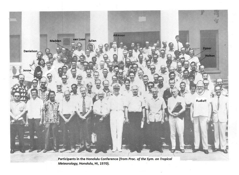
Figure 3Participants of the Honolulu Tropical Meteorology Conference in 1970 (photo credited to the American Meteorological Society and World Meteorological Organization, 1970). The key to all individuals in the photo can be seen in the AMS/WMO reference or in the Bulletin of the American Meteorological Society supplementary material (Madden, 2019).
In the discussion that followed my talk, Gary Atkinson from the U.S. Air Force made the observation that the nascent spectral studies of the tropics had been based on relatively short time series (the LIE time series were only 47 d long). He suggested that there were now long time series available from Pacific stations, and it would be good to compute spectra based on them to better assess the “variability and/or stability” (Atkinson, 1970) of results. We knew that Gary Atkinson was right, and Paul Julian and I were in the perfect position to look at longer time series. The NCAR Data Support Section headed by Roy Jenne had begun to collect some of these long series. Paul Julian had a FFT code based on Cooley and Tukey's 1965 algorithm, and we had access to a Control Data Corporation (CDC) 6600 device (Fig. 4). The CDC 6600 had a clock speed of 10 MHz and a memory of 65 KB, with a 60-bit word (NCAR, 2022), which, though orders of magnitude slower and smaller than a modern cell phone, made it the most powerful computer available for meteorological research at the time. Upon our return from Honolulu, I turned my attention to investigating the longest time series available from the equatorial region.

Figure 4CDC 6600 (© UCAR).
3.2 Studying longer time series
3.2.1 MJ71
Our motivation was to examine time variation in the spectra of tropical observations in the 4–5 d period range. The longest record available for this purpose was rawinsonde data from 3584 d measured at Canton Island (3∘ S, 172∘ W; now Kanton Island). With the long record, we could resolve lower-frequency variations that had not yet been investigated. Almost immediately, our attention shifted from documenting time variations in 4–5 d disturbances to investigating variations in the 40–50 d range because of results typified by Fig. 5. The coherence squared shown in Fig. 5 is similar to correlation as a function of frequency. It shows a broad maximum with largest values in the 40–50 d range. Corresponding phase angles (not shown) indicated that surface pressures and 850 hPa u winds were in-phase and 850 and 150 hPa u winds were out-of-phase.
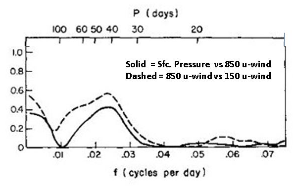
Figure 5Coherence squared between 850 and 150 hPa u winds (dashed) and between surface pressure and the 850 hPa u winds (solid), based on Kanton Island pressure and upper-air data. The 0.1 % prior confidence level, assuming a null of no coherence, is 0.25 (adapted from MJ71).
We had no a priori reason to expect this result, so the usual statistical tests were not appropriate. Paul Julian discussed prior versus posterior statistical tests in the paper we prepared (MJ71) and demonstrated that it would be rare to have such high coherence values if the time series were not related. He expanded on this argument in his paper published in 1971 (Julian, 1971).
Considering phase angles between participating variables, we concluded that the evidence pointed to a large-circulation cell oriented in the equatorial plane with a node where the u wind switches direction in the 600–500 hPa region. Neither the spectra nor the cross-spectra involving the v wind showed maxima in the 40–50 d range, so we concluded that it was not involved. We will see that data from more stations confirmed that the oscillation was indeed the manifestation of large circulation cells, but because none of our spectra differentiated between seasons, our conclusion about v wind was wrong.
The paper describing the results from Kanton Island was submitted to the Journal of the Atmospheric Sciences on 21 December 1970. A letter dated 12 March 1971 from the editor, S. I. Rasool, stated that the peer reviews, plural, were in, but relatively minor comments from only one reviewer were attached. We addressed the reviewer's comments, and the paper was published in July 1971 (MJ71).
3.2.2 MJ72
Working to obtain a full picture of the phenomenon that we were seeing at Kanton Island, we assembled station pressure data from 25 tropical stations (16 were within 15∘ of the Equator) and upper-air data from six stations all located within 15∘ of the Equator and spaced around its full circumference. Cross-spectra of the pressure data revealed that the 40–50 d disturbance propagated eastward and spread poleward but was strongest within 10∘ of the Equator. Based on cross-spectra of upper-air data from the six stations, we made a figure that summarized the status at all stations and levels that were coherent with Kanton Island pressure when Kanton Island pressure was a relative maximum (Fig. 6 in MJ72). That helped us to envision the zonally oriented circulation cells and their eastward movement.

Figure 6Two programmers (left) submitting their card decks to the operator for reading into the CDC 6600 in about 1970 (© UCAR).
To supplement the spectral evidence with a synoptic picture of the disturbance based directly on time series data, we turned to data from the International Geophysical Year, 1957–1958 (IGY). Willy Rudloff had presented a paper at the Honolulu Conference titled “Measurable Seasonal Variations in the Total Mass of the Atmosphere” (Rudloff, 1970), which was based on grid point pressure data digitized from IGY world weather maps prepared by his office, the Seewetteramt, in Hamburg. I wrote to him on 12 March 1971 about our interest in the tropical zone, and he kindly sent us the grid point sea level pressure data on computer cards, which was a standard way of storing and transferring data. We also tabulated and prepared punched cards containing IGY upper-air data from printouts available in the NCAR library. In 1970, all of our programs and much of our data were contained on punch cards. Typical of the time, Fig. 6 shows two NCAR programmers submitting their card decks into the CDC 6600 to be read.
We computed a composite wave by first selecting dates during the IGY period when 45 d band-pass-filtered Kanton Island pressure was at a relative minimum and then separately at a maximum and at six more intermediate times. The IGY data were then averaged for each of the set of eight dates separately. A pictured emerged that was consistent with the spectral results. The sea level pressure perturbations moved eastward, as did those of the zonal wind. There was a wave on the tropopause and some evidence of water vapor mixing ratio variations consistent with eastward-moving deep convection. A more detailed discussion of the first time we saw eastward propagation in the IGY pressures is contained in Hand (2015).
This spectral and synoptic evidence led to a description of the 40–50 d oscillation that is contained in Fig. 7. Phase E corresponds to the time when the station pressure is a relative maximum at Kanton Island and Phase A when it is a minimum. We had no precipitation or cloud data at the time but included an indication of the varying convection because of the low-level convergence in the u wind, mixing ratio changes, and the changing height of the tropopause.
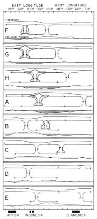
Figure 7Schematic depiction of the time and space variations in the oscillation. Phase A (E) is the time of lowest (highest) pressure at Kanton Island. Other phases are intermediate times and, for a 48 d period, are approximately 6 d apart. Anomaly pressures are indicated at the bottom of each panel, with negative anomalies shaded. Circulation cells are based on u-wind variations. Regions of enhanced convection are proposed based on u-wind convergence/divergence, tropopause height differences (top line), and mixing ratio changes.
We submitted our paper, describing the above results, on 6 April 1972. Editor S. I. Rasool, in a letter dated 8 May 1972, stated that “your paper has been found acceptable for publication”. This time, comments from two reviewers were included. Reviewer 1 accepted the paper on the condition that results from Gan island (0.7∘ S, 73.2∘ E) were included. Reviewer 1 stated that “Gan Island is strongly affected by the Asian Monsoon which seems to possess a 30–40 day period”. This was a qualitative assessment which was quantitatively documented by Yasunari (1979, 1980).
Fortunately, during the review process, we had begun to examine spectra and cross-spectra for Gan data, and the results were easily added to Figs. 1 and 4 of MJ72. Reviewer 2 gave us eight constructive comments which required only small changes. The paper was published in September 1972. We pointed out that the oscillation was a broadband one but called it the “40–50 day oscillation” because spectral maxima of the various variables most often fell in that range. The “MJO” reference began being used more frequently after it appeared in the title of two papers (Swinbank et al., 1988; Lau et al., 1988).
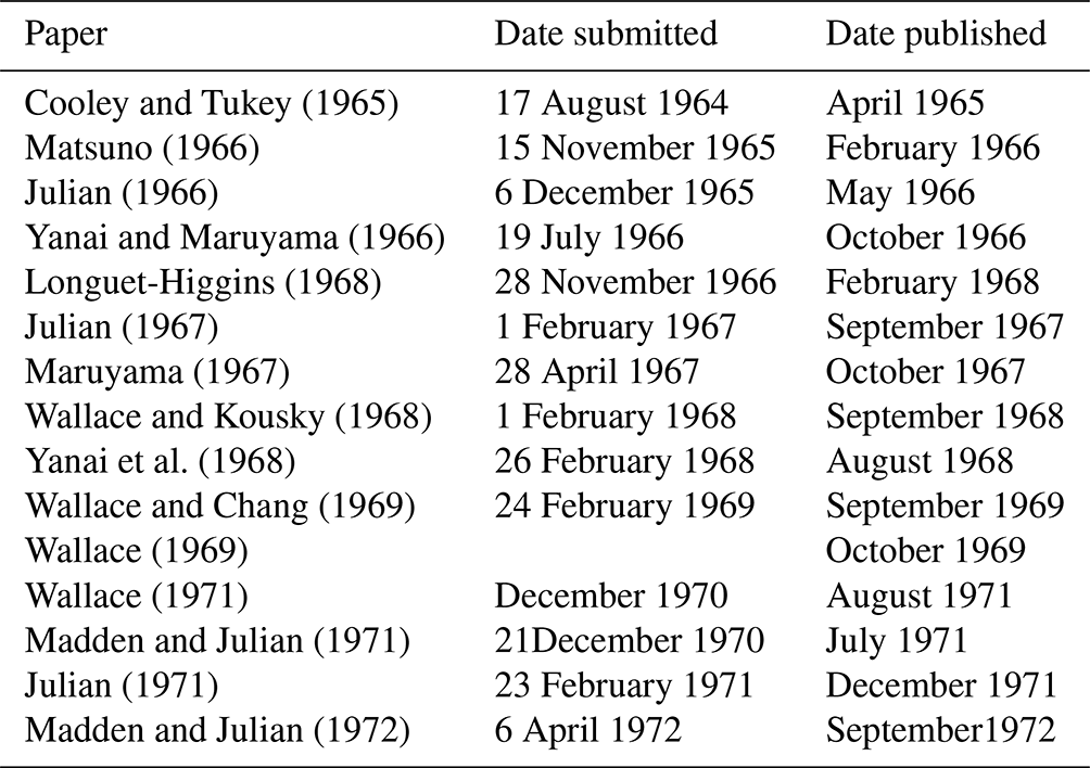
Table 1 shows the sequence of submission and publication dates for some of the relevant papers. Recently, Li et al. (2018) have brought to the attention of the international meteorology community a paper relating low-latitude basic flow and the occurrence of typhoons, written in Chinese and already published in 1963, that shows MJOs in the zonal wind during the 1958–1960 period. In the paper, which is not listed in Table 1 but is now a part of the history, Xie et al. (1963) observed that the u wind exhibited an oscillatory period of about 1.5 months.
Table 1Chronology of some relevant papers ordered by submission date.
4.1 Developments related to two of our conclusions
The clouds in Fig. 7 were based on circumstantial evidence. During the decade after MJ72, published papers using a wavenumber–frequency analysis of satellite brightness data (Gruber, 1974; Zangvil, 1975), case studies and spectral analysis (Yasunari, 1979, 1980), and compositing (Julian and Madden, 1981) provided evidence of cloud behavior consistent with Fig. 7.
Second, we concluded in MJ71 that the spectral results suggested that the v wind was not involved in the oscillation. Specifically, coherence squares between the v wind and u wind were not significantly different from zero. Some 15 years later, we learned that u and v are coherent and out-of-phase in Northern Hemisphere winter and coherent and in-phase in Northern Hemisphere summer. This in- and out-of-phase switch between seasons resulted in small cospectra and a resulting small coherence when, in MJ71, we averaged over the entire year. The seasonal-phase variations are consistent with surges in the wind from summer to winter hemispheres (see arguments in Madden, 1986).
4.2 Reception of MJ71 and MJ72
From 1972 through 1979, MJ71 and MJ72 were cited 17 and 19 times, respectively, according to the Web of Science. It is interesting to note that five of the MJ71 citations did not mention the oscillation itself but instead they referenced the spectral analysis method or Paul Julian's discussion about posterior statistical tests. Jim Holton at the University of Washington found the oscillation interesting, and in a letter to me shortly after MJ71 appeared, he offered prescient ideas about its spatial structure based on some of his modeling work (see Wallace, 2014); these were ideas which, unfortunately, we did not follow up on.
Interest in the two papers picked up in the 1980s, when MJ71 and MJ72 were cited 136 and 140 times, respectively. A circumstance that led to increased interest was the summer Monsoon Experiment (MONEX) during May through July of 1979. The MJO was active during that period (e.g., Krishnamurti and Subrahmanyam, 1982).
The path to the initial description of the MJO starts with the discovery of the QBO in 1961. The QBO stimulated studies aimed at explaining its remarkable behavior. These studies applied spectral analysis in innovative ways to describe tropical waves. The availability of relevant data was increasing, along with the computer power needed for efficient analyses. The fast Fourier transform, which sped up spectral calculations, was first coded for computers in mid-1960. The descriptions contained in MJ71 and MJ72 relied on the power of spectral analysis.
Considerable advances in the understanding of the MJO have been made in the 50 intervening years since MJ72. For up-to-date information, look at the following:
-
WGNE MJO Task Force – a Working Group of the WMO – available at https://wgne.net/activities/on-going-activities/wgne-mjo-task-force/ (last access: 9 February 2023);
-
MJO work at the United States Climate Prediction Center, available at https://www.cpc.ncep.noaa.gov/products/precip/CWlink/MJO/mjo.shtml (last access: 9 February 2023);
-
MJO monitoring and research at Australian Bureau of Meteorology (BOM), available at http://www.bom.gov.au/climate/mjo/ (last access: 9 February 2023);
-
S2S Prediction Project, available at http://s2sprediction.net/ (last access: 9 February 2023).
All the software discussed here was coded on punch cards more than 50 years ago and has long since been recycled. Moreover, data were assembled over 50 years ago on punch cards and magnetic tapes that are no longer available. No other data sets have been used in this paper.
The author has declared that there are no competing interests.
Publisher’s note: Copernicus Publications remains neutral with regard to jurisdictional claims in published maps and institutional affiliations.
This material was first prepared for a Zoom-based lecture at the University of Hamburg in December 2021 at the invitation of Nedjeljka Zagar. I thank Laura Hoff, of the NCAR Library, for her help. George Kiladis, Kathleen Madden, and Klaus Weickmann provided helpful comments on an early version of the paper, as did two anonymous reviewers. Most important, without Paul Julian's knowledge, insights, and generosity, MJ71 and MJ72 would not have been written.
This paper was edited by Kevin Hamilton and reviewed by two anonymous referees.
American Meteorological Society (AMS) and World Meteorological Organization (WMO): Proceedings of the Symposium on Tropical Meteorology, University of Hawaii, Honolulu, USA, 2–11 June 1970.
Atkinson, G. : Discussion following R. A, Madden’s paper, Wave Disturbances over the equatorial Pacific during the Line Islands Experiment, in: Proceedings of the Symposium on Tropical Meteorology, University of Hawaii, Honolulu, 2–11 June 1970, AMS/WMO, 1970.
Cooley, J. W.: The re-discovery of the fast Fourier transform algorithm, Microchim. Acta, 3, 33–45, 1987.
Cooley, J. W. and Tukey, J. W.: An algorithm for the machine calculations of complex Fourier series, Math. Comput., 19, 297–301, 1965.
Deland, R. J.: Some observations of the behavior of spherical harmonic waves, Mon. Weather Rev., 93, 307–312, 1965.
Ebdon, R. A.: Some notes on the stratospheric winds at Canton Island and Christmas Island, Q. J. Roy. Meteor. Soc., 87, 322–331, 1961.
Eliasen, E. and Machenhauer, B.: A study of the fluctuations of atmospheric planetary flow patterns represented by spherical harmonics, Tellus, 17, 220–238, 1965.
Eliasen, E. and Machenhauer, B.: On the observed large-scale atmospheric wave motions, Tellus, 21, 149–165, 1969.
Graystone, P.: Meteorological Office Discussion – Tropical Meteorology, Met. Mag., 88, 113–119, 1959.
Gruber, A.: Wavenumber-frequency spectra of satellite measured brightness in Tropics, J. Atmos. Sci., 31, 1675–1680, 1974.
Hand, E.: The Storm King, Science, 350, 22–25, 2015.
Haurwitz, B.: The motion of atmospheric disturbances, J. Mar. Res., 3, 35–50, 1940a.
Haurwitz, B.: The motion of atmospheric disturbances on the spherical earth, J. Mar. Res., 3, 254–267, 1940b.
Hough, S. S.: On the application of harmonic analysis to the dynamical theory of tides II. On the general integration of LaPlace's tidal equations, Philos. T. Roy. Soc. A, 191, 139–185, 1898.
Julian, P. R.: The Index Cycle: a cross-spectral analysis of zonal index data, Mon. Weather Rev., 94, 283–293, 1966.
Julian, P. R.: Variance spectrum analysis, Water Resour. Res., 3, 831–845, 1967.
Julian, P. R.: Some aspects of the variance spectra of synoptic scale tropospheric wind components in mid-latitudes and in the tropics, Mon. Weather Rev., 99, 954–965, 1971.
Julian, P. R. and Madden, R. A.: Comments on a paper by T. Yasunari, a quasi-stationary appearance of 30 to 40-day period in cloudiness fluctuations during the summer monsoon over India, J. Meteorol. Soc. Jpn., 59, 435–437, 1981.
Krishnamurti, T. N. and Subrahmanyam, D.: The 30–50 day mode at 850 mb during MONEX, J. Atmos. Sci., 39, 2088–2095, 1982.
Kubota, S. and Iida, M.: Statistical characteristics of atmospheric disturbances, Pap. Meteorol. Geophys. 5, 22–34, 1954.
Lau, N. C., Held, I. M., and Neelin, J. D.: The Madden-Julian Oscillation in an idealized general circulation model, J. Atmos. Sci., 45, 3810–3832, 1988.
Li, T., Wang, L., Peng, M., Wang, B., Zhang, C., Lau, W., and Kuo, H.-C.: A paper on the tropical intraseasonal oscillation published in 1963 in a Chinese journal, B. Am. Meteorol. Soc., 100, 1765–1779, 2018.
Longuet-Higgins, M. S.: The Eigen functions of LaPlace's tidal equations over a sphere, Philos. T. Roy. Soc. A, 262, 511–607, 1968.
Madden, R. A.: Wave disturbances over the equatorial Pacific during the Line Islands Experiment, in: Proceedings of the Symposium on Tropical Meteorology, University of Hawaii, Honolulu, 2–11 June 1970, AMS/WMO, 1970.
Madden, R. A.: Seasonal variations of the 40–50 day oscillation in the tropics, J. Atmos. Sci., 43, 3138–3158, 1986.
Madden, R. A.: How I learned to love normal-mode Rossby-Haurwitz Waves, B. Am. Meteorol. Soc., 100, 503–511, 2019.
Madden, R. A. and Julian, P. R.: Detection of a 40-50 day oscillation in the zonal wind in the tropical Pacific, J. Atmos. Sci., 28, 702–708, 1971.
Madden, R. A. and Julian, P. R.: Description of global-scale circulation cells in the tropics with a 40-50 day period, J. Atmos. Sci., 29, 1109–1123, 1972.
Madden, R. A., Zipser, E. J., Danielson, E. F., Joseph, D. H., and Gall, R.: Rawinsonde data obtained during the Line Island Experiment, Vol. I: Data reduction procedures and thermodynamic data, Vol. II: Wind data, NCAR Technical Note TN/STR-55, University Corporation for Atmospheric Research, https://doi.org/10.5065/D6W95737, 1971.
Maruyama, T.: Large-scale disturbances in the equatorial lower stratosphere, J. Meteorol. Soc. Jpn., 45, 391–408, 1967.
Matsuno, T.: Quasi-geostrophic motions in the equatorial area, J. Meteorol. Soc. Jpn., 44, 25–43, 1966.
NCAR Supercomputing history: https://www2.cisl.ucar.edu/ncar-supercomputing-history (last access: 9 February 2023), 2022.
Palmer, C. E.: Tropical Meteorology, Q. J. Roy. Meteor. Soc., 78, 126–164, 1952.
Panofsky, H. A.: Meteorological applications of power-spectrum analysis, B. Am. Meteorol. Soc., 36, 163–166, 1955.
Petterssen, S.: Weather Analysis and Forecasting, McGraw-Hill Book Co., Inc., New York, Library of Congress Catalog Card Number: 55-11568, 428 pp., 1956.
Reed, R. J., Campbell, W. J., Rasmussen, L. A., and Rogers, D. G.: Evidence of a downward-propagating annual wind reversal in the equatorial stratosphere, J. Geophys. Res., 66, 813–818, 1961.
Rossby, C.-G. and Collaborators: Relations between variations in the intensity of the zonal circulation of the atmosphere and the displacements of the semipermanent centers of action, J. Mar. Res., 2, 38–55, 1939.
Rudloff, W.: Measurable seasonal variations in the total mass of the atmosphere, Proceedings of the Symposium on Tropical Meteorology, University of Hawaii, Honolulu, USA, 2–11 June 1970, AMS/WMO, 1970.
Swinbank, R., Palmer, T. N., and Davey, M. K.: Numerical simulation of the Madden and Julian Oscillation, J. Atmos. Sci., 45, 774–778, 1988.
Thomson, W.: On gravitational oscillations of rotating water, P. Roy. Soc. Edinb., 10, 92–100, 1879.
Wallace, J. M.: Some recent developments in the study of tropical wave disturbances, B. Am. Meteorol. Soc., 50, 792–799, 1969.
Wallace, J. M.: Spectral studies of tropospheric wave disturbances in the tropical western Pacific, Rev. Geophys. Space Phys., 9, 557–612, 1971.
Wallace, J. M.: James R. Holton National Academy of Sciences Biographical Memoirs, National Academy of Science, 27 pp., http://www.nasonline.org/publications/biographical-memoirs/memoir-pdfs/holton-james.pdf (last access: 9 February 2023), 2014.
Wallace, J. M. and Chang, C.-P.: Spectrum analysis of large-scale wave disturbances in the tropical lower troposphere, J. Atmos. Sci., 26, 1010–1025, 1969.
Wallace, J. M. and Kousky, V. E.: Observational evidence of Kelvin waves in the tropical stratosphere, J. Atmos. Sci., 25, 900–907, 1968.
Xie, Y.-B., Chen, S. J., Zhang, I.-L., and Hung, Y.-L.: A preliminary statistic and synoptic study about the basic currents over southeastern Asia and the initiation of Typhoons, Acta Meteor. Sin., 33, 206–217, 1963 (in Chinese).
Yanai, M. and Maruyama, T.: Stratospheric wave disturbances propagating over the equatorial Pacific, J. Meteorol. Soc. Jpn., 44, 291–294, 1966.
Yanai, M., Maruyama, T., Nitta, T., and Hayashi, Y.: Power spectra of large-scale disturbances over the tropical Pacific, J. Meteorol. Soc. Jpn., 46, 308–323, 1968.
Yasunari, T.: Cloudiness fluctuations associated with the Northern Hemisphere Summer Monsoon, J. Meteorol. Soc. Jpn., 57, 227–242, 1979.
Yasunari, T.: A quasistationary appearance of 30 to 40 day period in the cloudiness fluctuations during the Summer Monsoon over India, J. Meteorol. Soc. Jpn., 58, 225–229, 1980.
Zangvil, A.: Temporal and spatial behavior of large-scale disturbances in tropical cloudiness deduced from satellite brightness data, Mon. Weather Rev., 103, 904–920, 1975.
Zipser, E. J.: The Line Islands Experiment, its place in tropical meteorology and the rise of the fourth school of thought, B. Am. Meteorol. Soc., 51, 1136–1146, 1970.