History of the Super Dual Auroral Radar Network (SuperDARN)-I: pre-SuperDARN developments in high frequency radar technology for ionospheric research and selected scientific results

Part I of this history describes the motivations for developing radars in the high frequency (HF) band to study plasma density irregularities in the F region of the auroral zone and polar cap ionospheres. French and Swedish scientists were the first to use HF frequencies to study the Doppler velocities of HF radar backscatter from F-region plasma density irregularities over northern Sweden. These observations encouraged the author of this paper to pursue similar measurements over northeastern Alaska, and this eventually led to the construction of a large HF-phased-array radar at Goose Bay, Labrador, Canada. This radar utilized frequencies from 8–20 MHz and could be electronically steered over 16 beam directions, covering a 52^∘ azimuth sector. Subsequently, similar radars were constructed at Schefferville, Quebec, and Halley Station, Antarctica. Observations with these radars showed that F-region backscatter often exhibited Doppler velocities that were significantly above and below the ion-acoustic velocity. This distinguished HF Doppler measurements from prior measurements of E-region irregularities that were obtained with radars operating at very high frequency (VHF) and ultra-high frequency (UHF). Results obtained with these early HF radars are also presented. They include comparisons of Doppler velocities observed with HF radars and incoherent scatter radars, comparisons of plasma convection patterns observed simultaneously in conjugate hemispheres, and the response of these patterns to changes in the interplanetary magnetic field, transient velocity enhancements in the dayside cusp, preferred frequencies for geomagnetic pulsations, and observations of medium-scale atmospheric gravity waves with HF radars.

1 Introduction

1.1 Motivation

During most of the 20th century, radar backscatter investigations of electron-density irregularities in the Earth's ionosphere were carried out predominantly with VHF (very high frequency) and UHF (ultra-high frequency) radars (e.g., Harang and Landmark, 1954; Leadabrand et al., 1965; Unwin, 1966; Ecklund et al., 1975; Greenwald et al., 1978). For measurements made at auroral zone and polar cap latitudes, observations were made at E-region heights (95–125 km). The objective of this early research was primarily to understand the physical processes that produce the irregularities. An early result of this research was that backscatter from ionospheric irregularities was only detected from those regions of the E-region ionosphere where the radar transmissions were directed within 2^∘ of normal to geomagnetic field lines. This led to the concept of aspect angle sensitivity (e.g., Unwin, 1966) and allowed researchers with VHF and UHF radars and magnetic field models to calculate the directions, ranges, and altitudes in which they could detect backscatter from these irregularities. These calculations were only possible for VHF and UHF radars since these frequencies undergo very little refraction as they transit the ionosphere and allow aspect angle analysis to assume straight-line propagation. An important result from these calculations was that it was impossible for radars located above 60^∘ magnetic latitude to detect backscatter from irregularities in the F region of either the auroral zone or polar cap ionosphere.

In the early 1960s, Buneman (1963) and Farley (1963) presented similar theories suggesting that field-aligned irregularities could be created by plasma streaming instabilities that were active at E-layer altitudes (95–125 km) and caused by electrons streaming at $(E\times B)/B^{\mathrm{2}}$ through the ion gas. Since the 1960s, additional plasma instabilities have been found to be capable of producing electron density irregularities in both the E and F regions of the ionosphere. These instabilities depend on the ionospheric electric field and plasma density and/or temperature gradients. In almost all cases, these instabilities produce irregularities that are extended along geomagnetic field lines and only observable if the radar wave vector in the scattering volume is orthogonal to the geomagnetic field. While the nature of these instabilities is of interest, it is beyond the intended scope of this history. Interested readers are referred to Fejer and Kelley (1980).

In the 1970s, I became involved with radar investigations of plasma instabilities in the auroral zone ionosphere over Alaska, and in 1975, I accepted a research position at the Max Planck Institut für Aeronomie (MPAe), where I led the development of the Scandinavian Twin Auroral Radar Experiment (STARE). STARE was an advanced pair of VHF radars, each operating at a specific frequency in the vicinity of 140 MHz. These radars were located near Trondheim, Norway, and Hankasalmi, Finland, and shared a large common viewing area extending over northwestern Norway and northern Sweden. The radars operated in a bistatic mode, transmitting on two vertical stacks of four Yagi antennas and receiving on a nearby array composed of 16 vertical stacks of four Yagi antennas. A unique feature of the STARE radars is that the signals received by the 16 Yagi stacks were input to a 16-port Butler phasing matrix that transformed the received signals into simultaneous returns from 16 beam directions. To avoid sidelobes, only the central eight beams of the matrix were used. The radar was operated in a single-pulse, double-pulse mode, with the single pulse providing the backscattered power profile and the double pulse providing the mean Doppler velocity profile for each beam. It was possible to process all backscatter returns from 400 to 1200 km in range and eight different viewing directions every 5–60 s, depending on integration time. When the data from the two radars were combined, it was possible to observe the circulation patterns of ionospheric irregularities over the entire field of view. Further technical details are given in Greenwald et al. (1978), while a summary of some of the scientific results is given in Nielsen and Schmidt (2014).

In time, however, it became apparent that there were an unacceptably large number of returns that exhibited Doppler velocities in the vicinity of the ion-acoustic velocity. The linear theory of the two-stream instability predicts that the instability will be excited when the relative electron ion drift velocity equals the ion-acoustic velocity, but that the phase velocity of the unstable modes will continue to track the electron drift velocity if it exceeds the ion-acoustic velocity. Unfortunately, this does not appear to be the case. The dominant unstable modes appear to be observed at the threshold of the instability and remain at that velocity. Similar results had been observed previously by VHF radars located under the equatorial electrojet and by VHF and UHF radar investigations at other auroral zone locations. Numerous theorists have tried to explain this phenomenon, but no one has provided a widely accepted explanation. Nielsen and Schmidt (2014) discuss this issue.

Later, in my tenure at MPAe, I had the opportunity to introduce French scientists from the Université de Toulon to Swedish scientists at the University of Uppsala. The Toulon group wanted to collaborate with the Swedes in the construction and operation of an HF radar near Uppsala, Sweden. Their radar used a linear array of eight tri-band antennas operating near 14, 21, and 28 MHz, and they proposed identifying the radar as SAFARI (Sweden And France Auroral Radar Investigation). This collaboration became operational about 1 year after my family and I had returned to the United States. The first observations included HF Doppler spectra obtained from F-region ionospheric irregularities over northern Scandinavia in November 1980 (Hanuise et al., 1981). Several years later, a more complete comparison of HF radar observations of F-region irregularity drifts and EISCAT incoherent scatter radar observations of F-region plasma drifts was reported by Villain et al. (1985).

The rationale for switching from VHF frequencies to HF frequencies results from differences between E- and F-region plasmas. At E-region heights, the electrons are essentially collisionless. In the presence of an electric field that is transverse to B, they undergo a Hall drift, $(E\times B)/B^{\mathrm{2}}$, in a direction that is orthogonal to both E and B. In contrast, the ions are bound by collisions to the neutral gases in the upper atmosphere. Above 140 km altitude, and particularly in the F region, the neutral gas density is substantially lower than in the E region, enabling ions and electrons to drift in their distinct Larmor orbits as a plasma at $(E\times B)/B^{\mathrm{2}}$. Instabilities due to plasma density and temperature gradients still produce ionospheric irregularities, but the two-stream instability and its characteristic spectral peak at the ion-acoustic velocity should not be observed.

With this thought in mind, I started to think seriously about using HF frequencies to study irregularities in the auroral zone and polar cap ionospheres. I realized that the HF frequencies we would use were only a factor of 2–3 greater than the peak plasma frequency of the F layer, and therefore, were very susceptible to refraction by the positive electron density gradient on the bottomside of the F region. The F₂ layer, which is the most ionized portion of the F layer, extends from 200 to 500 km in altitude. As the radar transmissions propagate upward into the F layer, the increasing electron density refracts the rays toward the horizontal direction and, in the process, causes them to pass through the range of angles where they are propagating within 2^∘ of orthogonal to the steeply inclined magnetic field lines in the high-latitude auroral zone and polar cap. If they encountered ionospheric irregularities while at these angles, backscattered signals would propagate along the reciprocal path and return to the radar site, while most of the energy in the transmission will continue to propagate upwards. If it passes through the peak of the F layer, it will enter the topside ionosphere and encounter a region of decreasing electron density, where the transmission will slowly return to its original propagation direction. In the process, it must again pass through a range of angles where it is propagating within 2^∘ of orthogonal to the geomagnetic field, and if ionospheric irregularities are again present, backscattered signals will be generated and follow the reciprocal path though the peak of the F layer and return to the radar site. Finally, there is a possibility that the radar transmission that passed through the orthogonal propagation zone in the bottomside ionosphere will be reflected by the ionosphere before reaching the topside. This reflected ray would then propagate downwards, recovering its original elevation angle as it emerges from the ionosphere and continues at that elevation angle until it strikes the Earth's surface. A portion of the incident energy that is scattered by the Earth's surface will return to the radar site via the reciprocal path, while the bulk of the energy will be reflected forward toward the ionosphere in a 1.5 hop propagation mode. Due to the ionosphere's ability to trap a significant fraction of the energy in each transmitted pulse within this Earth ionosphere wave guide, it appears that backscattered signals could be produced over a large set of ranges.

There is one final point regarding radar measurements at HF frequencies. HF radar transmissions at 10 and 20 MHz have wavelengths of 30 and 15 m, respectively. One can achieve reasonable azimuthal resolution by constructing a linear array of 16 antennas, but there is no easy way to construct an HF antenna array that has a narrow beamwidth in elevation. In fact, it is probably not desirable. For the Super Dual Auroral Radar Network (SuperDARN) antennas that I shall describe shortly, the peak transmitted power at 10 MHz is located at an elevation angle of ∼ 35^∘, and the vertical beamwidth of the transmission is ∼ 42^∘, while, at 18 MHz, the peak radiated power is at an elevation angle of ∼ 25^∘, and the vertical beamwidth of the transmission is ∼ 25^∘. Most of the angles that lie within these vertical beam patterns have the potential of passing through one or more zones of near-orthogonal propagation and contributing to the total backscattered signal.

The preceding thoughts reflect my feelings back in 1980, when I was trying to decide whether to continue VHF radar investigations of E-region irregularities or pursue a new path that would use HF frequencies to investigate F-region ionospheric irregularities at high latitudes and use them as tracers of plasma motions and electric fields in the high-latitude ionosphere. I was confident that I would obtain better measurements of plasma drifts from F-region irregularities, but I was also worried about the increased complexities of refraction and propagation that are associated with HF observations. In the end, I decided to pursue the HF backscatter path, because I felt that, if the effort were successful, the rewards would be far greater.

1.2 Early investigations of backscatter from the high-latitude F layer

In 1980, there were very few published papers on the topic of HF backscatter from high-latitude ionospheric irregularities. One of the earliest by Bates and Albee (1970) described observations of F-region irregularities over Alaska using a swept-frequency ionosonde. Near the end of 1980, Hanuise et al. (1981) carried out their initial measurements with the SAFARI radar located at Lycksele, Sweden. Their technique was to operate the radar at a low pulse repetition frequency (PRF) until they identified increased return power from some range. Then, they would increase the PRF until the transmitter pulses bracketed the identified target and was sampled with sufficient rapidity for the spectrum to be unaliased. Some of their spectra were peaked near the ion-acoustic velocity, but there were others that were clearly above the ion-acoustic velocity.

In the same period, a new, advanced HF ionospheric sounder had been deployed to a field site near Cleary Summit, Alaska. It was developed by the National Oceanic and Atmospheric Administration (NOAA) Space Environment Laboratory, with partial funding from the Atmospheric Sciences Directorate of the National Science Foundation (NSF). This instrument was designed primarily to measure electron-density profiles in the bottomside of the auroral zone ionosphere. However, NSF was also interested in adapting the instrument to other applications. One of these was to evaluate its potential for obtaining oblique backscatter soundings of E- and F-region irregularities in the auroral zone and polar cap ionospheres. I prepared a successful NSF grant proposal requesting funds to purchase four log-periodic antennas and towers and have them installed at the Cleary field site by the technical staff of the University of Alaska Fairbanks (UAF) Geophysical Institute.

Near the end of 1981, Jean-Paul Villain, of the Université de Toulon HF radar group, and I traveled to Alaska, where we carried out an initial campaign using the Cleary sounder and the new antenna array. Our plan was to obtain autocorrelation functions (ACFs) of radar signals backscattered by F-region irregularities in the auroral zone and polar cap ionospheres. These data would then be Fourier transformed to produce Doppler spectra. The ACFs would be obtained by transmitting multiple pairs of transmitter pulses, with each pair being an integral multiple of some basic lag. While we were able to detect ionospheric returns over a large-range interval, the computer controlling the Cleary ionosonde could not support the rapid changes in the double-pulse separation that were necessary to obtain quality ACFs. On our return flight to Maryland, Jean-Paul and I discussed the situation and concluded that a more efficient approach would be to use multipulse timing sequences of the type identified by Farley (1972) for incoherent scatter radar measurements. These sequences consist of bursts of 4–10 transmitter pulses, with spacings that could be used to calculate, without redundancy, most of the lags of an ACF. To be fair, it is possible that the computer used on the Cleary ionosonde could have produced a multipulse sequence if we did not attempt to change it rapidly, but there was no software on the Cleary computer or its front-end processor to calculate ACFs from multipulse sequences. For this reason, we decided to purchase a microcomputer, of the type used on the STARE radars in Scandinavia (Greenwald et al., 1978), with which we had significant programming experience. At JHU/APL (Johns Hopkins University Applied Physics Laboratory), internal research funding was provided to us to support this hardware and software development. In the end, the phase-coherent receiver and frequency synthesizer of the Cleary sounder were mated to the new microcomputer-based data acquisition and processing system, a 3 kW linear power amplifier, the new HF antennas and a phasing matrix that used sets of cables to form beams in specific viewing directions.

By the end of 1981, Jean-Paul had returned to France, while I continued to work on the software for acquiring, processing, and displaying the data from the Cleary sounder. The multipulse sequence that we used produced extended arrays of in-phase and quadrature data samples. These were input to the microcomputer and converted into ACFs. Within these arrays, the locations of the transmitter pulses were known, so it was relatively easy to select the in-phase and quadrature samples for each range gate and calculate each lagged product of the multipulse sequence. The multipulse sequence that we used enabled us to determine lags 0 through 16τ, where τ is the minimum non-zero lag. Lag 13 of the ACF was not used because it could be calculated by three different pulse pairs, which would have caused confusion.

In early February, all APL components of the HF radar were crated and shipped to the Cleary field site. I arrived there shortly after the middle of the month and reassembled the system. Preliminary testing of the HF radar confirmed that it could produce quality ACFs from ionospheric backscatter. During this initial campaign from Cleary, Alaska (AK), measurements with the HF radar were limited to the range interval from 975 to 1725 km, with a range resolution of 15 km. The objective was to detect mostly, if not solely, direct backscatter from F-region irregularities. Data acquisition began on 25 February and continued through 1 March 1982. The observations coincided with the final operations of the incoherent scatter radar at Chatanika, AK, which was then disassembled and transported to Sondrestrom, Greenland, where it has been in operation for more than 30 years. During these 5 d, the HF radar produced ∼ 700 000 ACFs, of which ∼ 10 % were associated with backscatter from ionospheric irregularities. Some observations are described in Greenwald et al. (1983).

1.3 Similarities and differences between STARE and HF radars

I have been asked to discuss the similarities and differences between STARE and SuperDARN. The main similarity between STARE and SuperDARN is that both radars were designed to run autonomously and continuously. This means that, in most cases, there was always STARE or SuperDARN data available for others in the research community. Often, it was for applications that we had not considered. I was especially happy about the work that students of Jürgen Untiedt, a professor at the Institut für Geophysik der Universität Münster, were able to carry out using STARE data and magnetometer data during the International Magnetospheric Study. I also appreciated the international response to the Goose Bay radar that enabled the rapid development of the SuperDARN network.

The consequences of going to HF frequencies are considerable. The ionosphere is very dynamic at high latitudes, and the amount of refraction that a packet of rays undergoes as it transits the ionosphere is substantial. It is important to know the elevation angles of the rays that are being backscattered by F-region irregularities, as this allows the ground range and refractive index of the scattering volume to be determined. With VHF and UHF radars, you know the rays travel in straight-line paths, and there is no refraction. If irregularities exist in a volume where you have good aspect angle, you will detect backscatter; otherwise, you will not.

SuperDARN uses large, horizontally polarized, log-periodic antennas mounted on top of 15.24 m galvanized steel towers. These antennas have an operating bandwidth of 8–20 MHz, which enables them to detect backscatter throughout the day and night over most of the solar cycle. The STARE transmitting antennas direct 50 kW of power into an azimuth sector of 30^∘, while the SuperDARN antennas radiate a combined power of 10 kW into a 2.5–6^∘ azimuth sector. The power densities of the transmission from these two systems would be comparable were it not for the fact that STARE radars have a vertical beamwidth of 10^∘ on both their transmitting and receiving arrays, while the SuperDARN antenna has a vertical beamwidth of 25–50^∘, depending on the operating frequency. Fortunately, the additional vertical beamwidth is beneficial when it comes to detecting backscatter at elevation angles greater than 30^∘.

Because the STARE radars operated at a single frequency, they can use a Butler phasing matrix. This is an elegant solution that Fourier transforms the signals from a 16-antenna array into simultaneous signals from 16 viewing directions. When viewed in color, it also looks like a piece of metal art. In contrast, HF radars must use time delay steering to form the antenna array beam directions. In the original Goose Bay radar, the time delays were provided by switches and lengths of cable stuffed into a large aluminum crate. Now, most radars, including Goose Bay, have advanced to using capacitive delay lines, and some are using digital frequency synthesizers.

In data processing, the STARE radars originally used alternating single-pulse, double-pulse sequences which provided range profiles of backscattered power and Doppler velocity, while SuperDARN radars use multipulse sequences to obtain ACFs of the backscattered signals. ACFs and Fourier transformed Doppler spectra may help to identify F-region instability processes.

Finally, SuperDARN radars must use an interferometer array to determine the elevation angles of backscatter signals. This information is essential for understanding the propagation path of each transmitted ray and the ground range to the location underlying each scattering volume. This topic will be discussed in more detail later in this history. Now, we return to 1982.

2 Construction of the Goose Bay HF radar

2.1 Original system

Upon returning to APL, I asked Kile Baker to process the data tapes from the Cleary campaign and produce Doppler spectra from the ACFs. While he was working on this, I considered future research activities that we might pursue. Knowing that the Air Force Geophysics Laboratory (AFGL) had an ionosonde site next to the airport in Goose Bay, Labrador, and that Goose Bay would also be an excellent site for collaborative measurements with the incoherent scatter radar that was being reinstalled near Sondrestrom, Greenland, I asked Herb Carlson and Jürgen Buchau of the Ionospheric Physics Branch of the Air Force Geophysics Laboratory (AFGL) if it were possible to install an HF radar on the ionosonde field site. They responded favorably, noting that HF radar measurements would complement the ionosonde measurements being made at the site. Their sole concern was possible radio interference between two instruments that operated in the same frequency band. We discussed ways the interference could be minimized and concluded that the potential for collaboration was worth the effort.

In July 1982, a proposal for the construction of an HF radar at Goose Bay, Labrador, was submitted to the Upper Atmospheric Sciences Division of the NSF and the Air Force Office of Scientific Research (AFOSR). Both funding agencies provided financial support for the project. Additional financial and/or labor support was provided by the Atmospheric Effects Division of the Defense Nuclear Agency (AFGL) and the Propagation Branch of the Rome Air Development Center (RADC), together with internal research and development support from JHU/APL. Funding for the construction of the Goose Bay radar became available in April 1983.

Most of the electronics for the original radar, including the phasing matrix, were fabricated in the electronics shops at JHU/APL. The phasing matrix was a large aluminum box that housed computer-controlled switches and eight sets of 16 coaxial cables. Each set of cables provided the time delays that were required to direct the beam into one of eight beam directions, and the switches were used to select the beam and whether the beam was directed to the left or right of the array normal direction. Including the beamwidth of the transmitted signals, the full width of the 16-beam scan was ∼ 52^∘, and the spacing between beams was 3.24^∘. More information on the phasing matrix and some theoretical beam patterns are found in Greenwald et al. (1985).

The original HF power amplifiers used on the Goose Bay radar were inexpensive commercial units purchased from a firm that produced HF communication systems for taxis in Asia. Each power amplifier operated in class AB and had an average output power of 125 W across our frequency band. When all components and cables for the Goose Bay radar were ready, everything was crated, transported to McGuire Air Force Base in New Jersey, and flown via military aircraft to Goose Bay, Labrador.

At the same time, parts for 16 antennas and towers were fabricated by Sabre Communications Corporation and shipped by truck and ferry to the AFGL field site near Goose Bay Airport, where a local contractor was constructing 16 concrete piers onto which the towers and antennas would be mounted. The cost for the original antennas, towers, and piers was ∼USD 70 000. The antennas and towers required complete assembly at the site, which began in September 1983 and was completed on 11 October 1983. This work was performed by J. Waaramaa, R. Galik, K. Degan, R. Gowell, and J. Winterbottom of AFGL, J. Kelsey, W. Conkie, and B. Gill of Canada Marconi (the local site crew for the Goose Bay ionosonde), R. Drake and T. Stevenson of the 438 MAW USAF (Military Airlift Wing of the United States Airforce), Mike Pinnock of the British Antarctic Survey, C. Hanuise of LSEET (Laboratoire de Sondages Electromagnétiques de l'​Environnement Terrestre), Université de Toulon, and K. B. Baker, R. A. Hutchins, and myself of JHU/APL. Fortunately, all construction work, aside from the JHU/APL group and the concrete work, was provided at no cost to our grant. Mike Pinnock was there to gain experience in the HF technology being used in preparation for a future proposal involving HF radars in Antarctica, while C. Hanuise was in the process of redeploying his HF radar instrumentation to Quebec, Canada. Preliminary assembly of the towers took place in an aircraft hangar. Each tower was fabricated from galvanized steel and comprised of two 6 m sections and one 3 m section. Each antenna was made of aluminum and was 12 m long. The length of the completed antenna array was ∼ 240 m (the STARE receiving array was 30 m in length).

Each SuperDARN antenna consisted of 10 dipole elements that are spaced logarithmically and cut for one of the frequencies in the 8–20 MHz band. The higher-frequency dipoles were toward the front of the antenna, and the lower-frequency dipoles were toward the rear. These antennas are inherently broadbanded and only the dipole element that was most resonant with the transmitter frequency, and its nearest neighbors are active at any time. The element in front of the most resonant element served as a director, and the element behind the most resonant element served as a reflector. Together, they directed the transmitted signal toward the high-frequency end of the antenna as it was radiated into space. These antennas were solidly constructed and have withstood the rigors of an arctic climate for over 35 years!

In the original Goose Bay radar, the HF amplifiers and transmit–receive ($T/R$) switches were mounted in galvanized steel enclosures bolted to the base of each antenna tower. At the center of the antenna array, a wooden equipment shed built on stilts housed the phasing matrix, power supplies, and switching circuitry for the transmitters and phasing matrix. This shed was ∼ 300 m from a concrete block building that housed the ionosonde electronics and computers, the HF radar computer, frequency synthesizers, HF radar receiver, and video display. The ionosonde typically operated for about 2 min every 15 min, so we scheduled a pause in radar operations for the duration of each sounding.

Figure 1 shows a photograph of the Goose Bay radar shortly after installation of the antennas. The red structure at the center of the array is the equipment shed that holds the power supplies, phasing matrix, and switching circuitry for the transmitters. The white building seen in the background, to the right of the red equipment shed, is the concrete block building housing the ionosonde and some of the HF-radar electronics and computers. It is 350 m beyond the center of the array. At the far end of the antenna array, one can see, above the white line, some of the transmitter units that have been mounted to the antenna towers. The remainder are resting on the concrete piers.

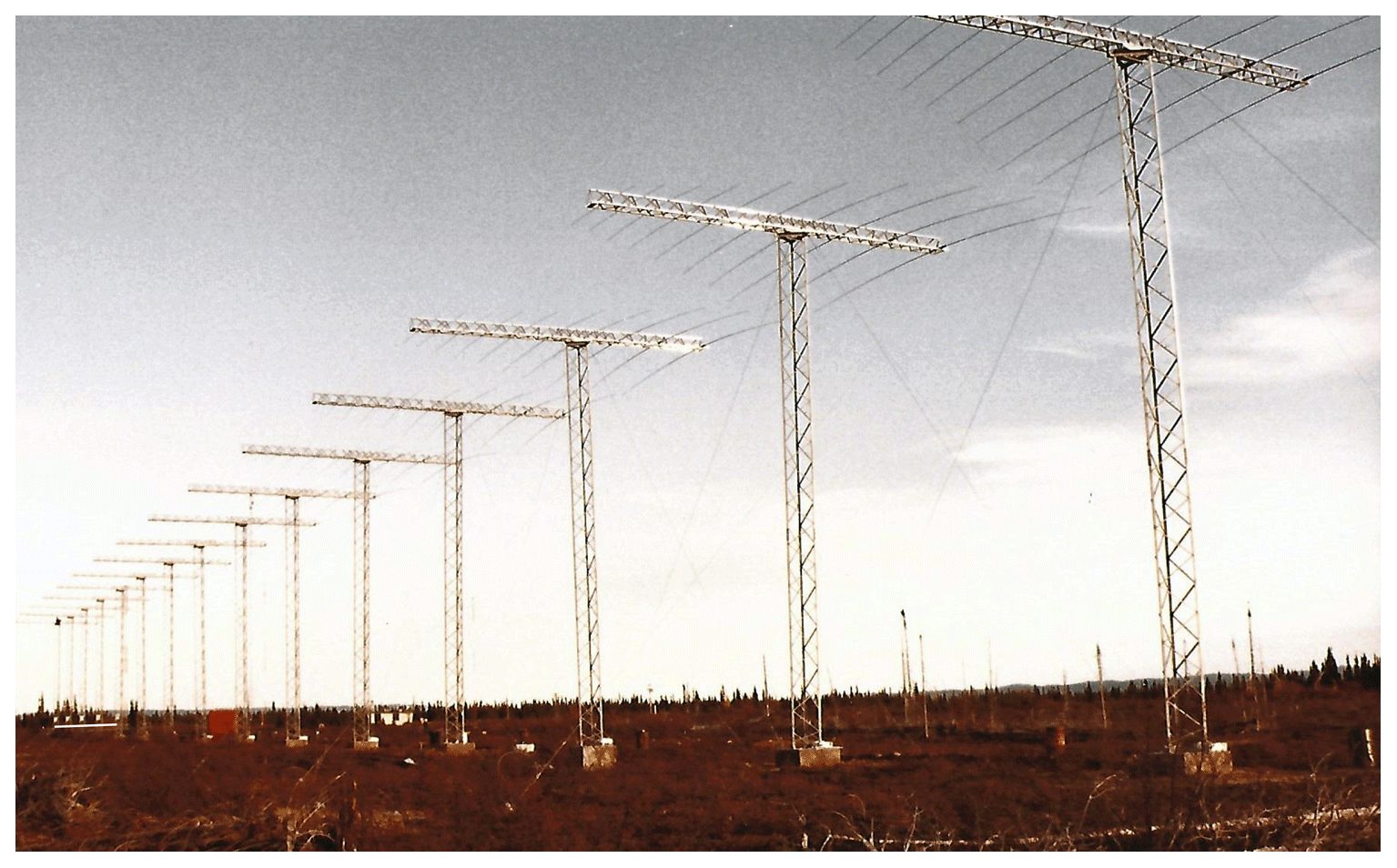
Figure 1 View of the Goose Bay HF antenna array after the towers and antennas were installed. The power radiated by the antennas is directed toward the left in this figure. Note the red equipment shed at the center of the array. It contains power supplies for the transmitters, the phasing matrix, and digital switches for controlling the pointing direction of the selected beam. To the right of the phasing shed is a white building that is located 350 m beyond the center of the array. This building contains the computers for controlling the radar and processing and displaying the acquired data. At the far end of the array, one can see that five of the transmitters have been mounted on the towers. The remainder are sitting on the concrete bases for the towers.

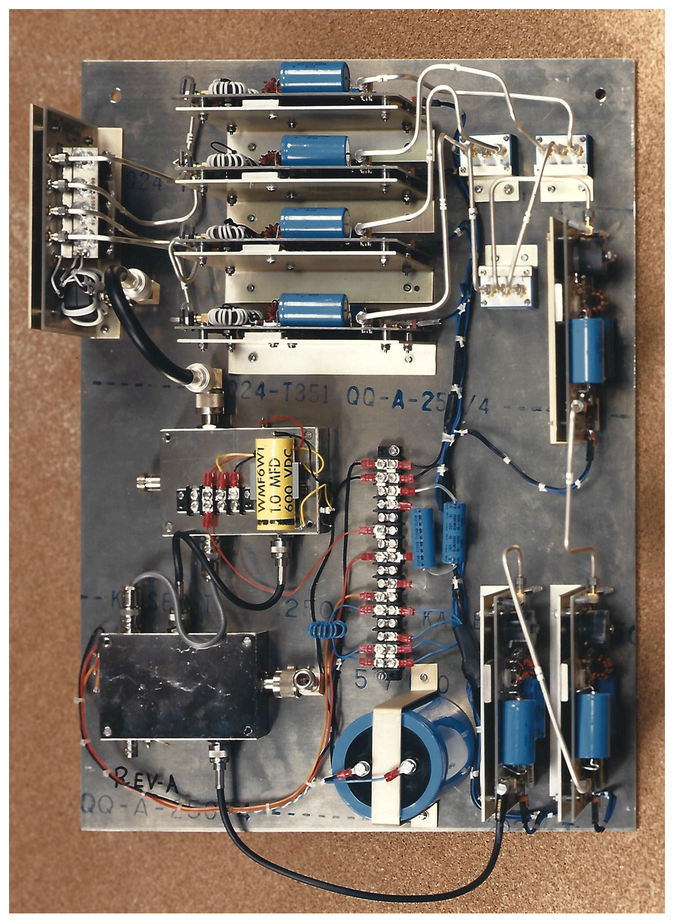
Figure 2 Photograph of one of the upgraded 800 W transmitters as they appeared in their galvanized steel containers. A total of four 200 W amplifier modules are stacked at the top of the plate, and their outputs are summed in the power combiner to the left. The output of the power combiner is connected to the high-power $T/R$ switch. During transmission, the forward power is directed to the open connector on the high-power switch, which is connected via cable to the antenna. On reception, the signals received by the antenna enter the high-power switch through the open connector and exit it through the connector immediately under the yellow capacitor. It then passes through the low-power switch, the phasing matrix, and back to the receiver in the control building. This photo was produced by the photography group at JHU/APL in 1986. It is identified as photo no. 220592.

As noted previously, transmissions from obliquely directed HF radars are refracted toward the horizontal direction by the positive electron density gradient below the peak of the F layer. Electron densities in the high-latitude ionosphere are controlled primarily by the extreme ultraviolet (EUV) radiation from the Sun, which has diurnal, seasonal, and solar cycle variability, and also by energetic particle precipitation. For obliquely directed transmissions, the radar-operating frequency should be a factor of 2–3 greater than the peak plasma frequency of the F layer. This allows some of the angles in the transmitted signal to achieve near-normal propagation to the geomagnetic field and a somewhat smaller set of angles to be reflected by the ionosphere.

The Goose Bay radar has been in almost continuous operation for nearly 37 years. The first paper was based on results obtained during the first few days of operation (Greenwald et al., 1985). It describes more completely the operation of the phasing matrix, theoretical beam patterns at several frequencies, and the nature of the multipulse sequence that was used. It also presents examples of some of the data products that were obtained, including real-time displays, ACFs, Doppler spectra, and 2-D scans of the signal-to-noise ratio (SNR) and Doppler velocity of the observed ionospheric irregularities.

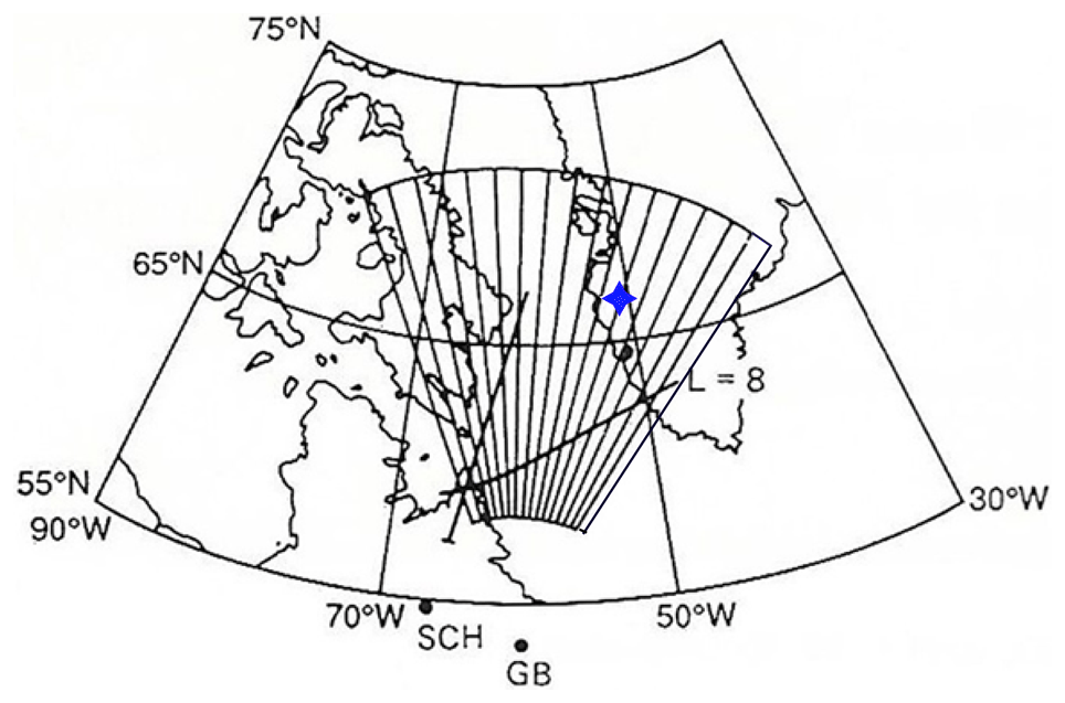
Figure 3 Map of northeastern Canada and southern Greenland. Superimposed on the map are the 16 beams of the Goose Bay (GB) radar. The line coming from the direction of Schefferville (SCH) radar represents the direction of the Schefferville beam, and the beamwidth is approximately twice that of a single Goose Bay beam. The blue star indicates the approximate location of the Sondrestrom incoherent scatter radar (ISR). The curved line identified as L=8 corresponds to slightly more than 69^∘ geomagnetic latitude. Adapted from Fig. 1 of Villain et al. (1990).

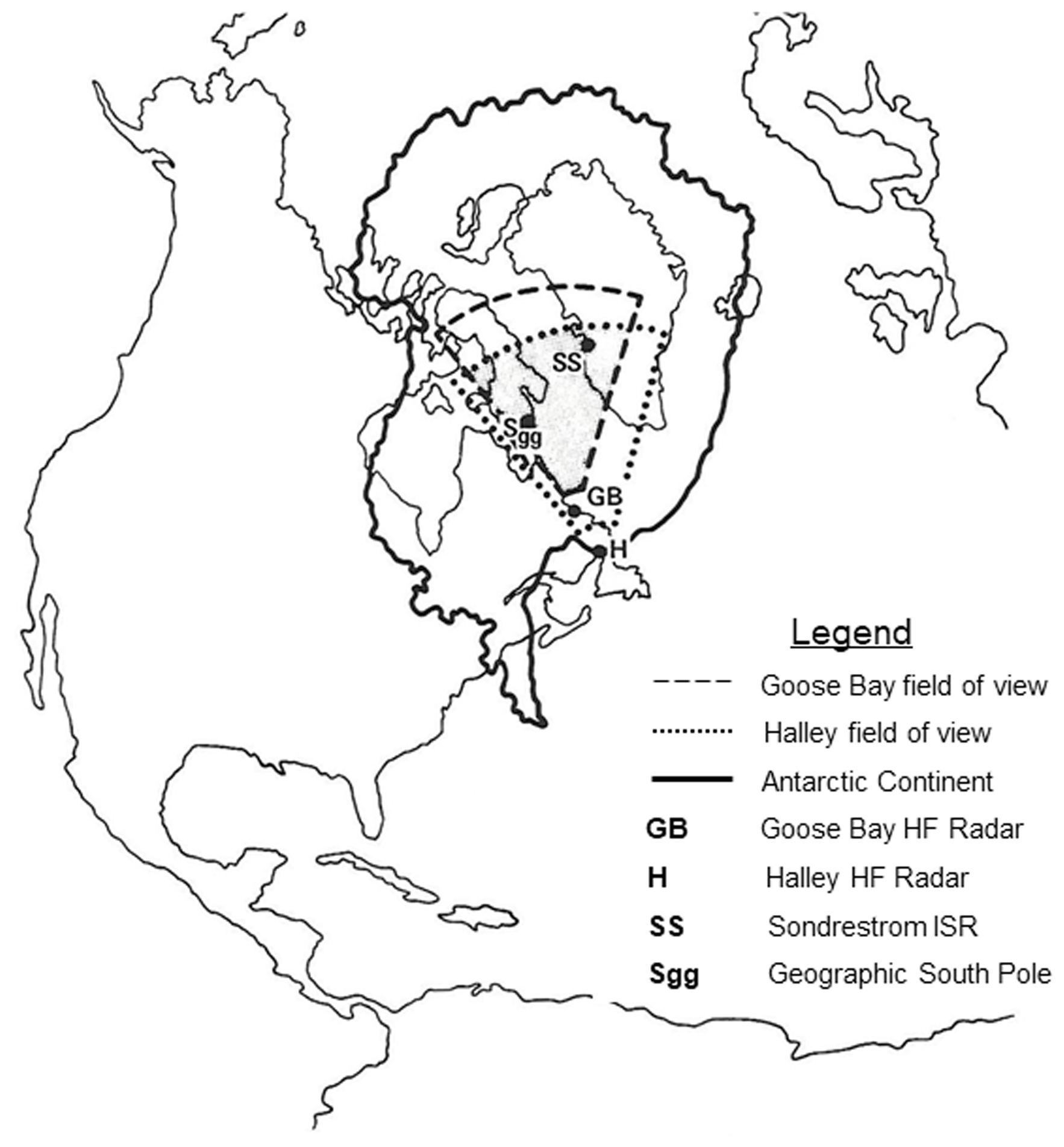
Figure 4 Map of the Northern Hemisphere upon which the magnetically conjugate regions of Antarctica are superimposed. The Northern Hemisphere land masses are bounded by the thin black lines, while the Antarctic continent is bounded by the bold black line. The Halley (H) HF Radar is near the coast of Antarctica, while the Goose Bay (GB) HF Radar is near the northeastern coast of Canada. Also indicated on the map are the nearly overlapping conjugate fields of view of the Goose Bay radar (bold dashed lines), the Halley radar (bold black dots). The location of the Sondrestrom Incoherent Scatter Radar (SS) and the mapped location of the Geographic South Pole (S_gg) are also indicated. This figure was originally produced by the British Antarctic Survey in support of a proposal to the Office of Polar Programs at the U.S. National Science Foundation. The proposal was entitled the Polar Anglo-American Conjugate Experiment (PACE).

The basic data products of the radar were 17 lag raw ACFs derived from quadrature output samples from the radar receiver. The raw ACFs and supporting operational parameters were stored on digital magnetic tape and shipped by Canadian and US mail to JHU/APL. At JHU/APL, the tapes were initially processed to remove bad lags due to the receiver being gated off or being subject to a strong return from an interfering signal. The remaining lags of the refined ACFs were then processed to produce a 32-point Doppler spectrum, and the mean Doppler velocity from each range gate was derived from the phase slope of the refined ACF as a function of lag, the SNR from the lag 0 power, and the coherence of the ACF from the decay in the backscattered power as a function of lag. ACFs from ground backscatter exhibit very low (often zero) Doppler shifts and very high coherence, while ACFs from ionospheric backscatter have much larger Doppler velocities and much lower coherence than ACFs from ground backscatter. Due to these differences, we were able to remove ground backscatter, so that it did not interfere with the calculation of ionospheric drift velocities.

2.2 Initial improvements

Even though the original Goose Bay radar worked well, there were a few areas where technical upgrades would significantly increase the amount and quality of the data. The first of these involved the replacement of the 125 W power amplifiers with 800 W power amplifiers (shown in Fig. 2). This power amplifier is comprised of four 200 W modules operating in parallel and followed by a four to one combiner. On transmit, the signal from the phasing matrix is gated through the amplifier chain along the bottom and right-hand side of the figure, through the power dividers in the upper right-hand corner, and then through the four parallel 200 W amplifiers to the four to one combiner. Next, the output signal passes through the high-power $T/R$ switch, which is the metal box topped with a yellow 600 V capacitor. During transmission, the RF (radio frequency) pulse exits the high-power $T/R$ switch through the open connector on the left side of the unit and travels via RF cable to the log-periodic antenna at the top of each tower. During reception, the signals backscattered from the ionosphere and Earth's surface are received by the log-periodic antennas and directed downward through the same cable to the galvanized steel box, where they pass through the high-power and low-power $T/R$ switches and exit through the open connector at the bottom left of the low-power $T/R$ switch, which leads through coaxial cables that return to the phasing matrix. There, the signals from the 16 antennas pass in the reverse direction through the phasing matrix and are subsequently summed in a 16-port combiner. This signal then propagates through the RF cable that extends between the equipment shed and the concrete block building. There, the backscattered signals pass through a narrow-band, phase-coherent receiver, are digitized, processed in the on-site computers, and recorded on digital tape.

One of the most important components of this entire system is the high-power $T/R$ switch. Due to the higher transmitted power levels of the new amplifiers, the high-power $T/R$ switches had to be completely redesigned. This switch, topped with the 600 V capacitor, must pass 1 kW of forward power to the antenna port, while maintaining 80 dB of isolation to its receiver port. If this level of isolation is not maintained, the power leaking back to the input of the low-power $T/R$ switch is sufficient to damage the amplifiers and $T/R$ switches in the transmitter units. The new design required significantly higher back-bias voltages on the pin diodes in the switch and has been used, with minor modifications, on most subsequent SuperDARN radars.

The final and potentially most important upgrade to the Goose Bay radar took place in the summer of 1984. Under support from RADC and AFGL, an additional array of 16 antennas and towers were purchased and transported to Goose Bay, where two teams of Massachusetts Air National Guard members assembled and erected them 100 m north of the original array. Both arrays receive backscattered signals from the ionosphere and the Earth's surface. The time difference between the arrival of the backscattered signal at each array is used to determine the elevation angle of each returning signal. Originally, we thought this information would allow us to identify the propagation mode of each backscattered signal, but we did not realize how important it really was. This point will be discussed in greater detail in the next part of this history.

Figure 5 Photograph taken in 1988, showing the main array of the Goose Bay radar, the 16-antenna interferometer array, and John Dudeney. John is standing about halfway between the center of the main array and the white building that was identified in Fig. 1.

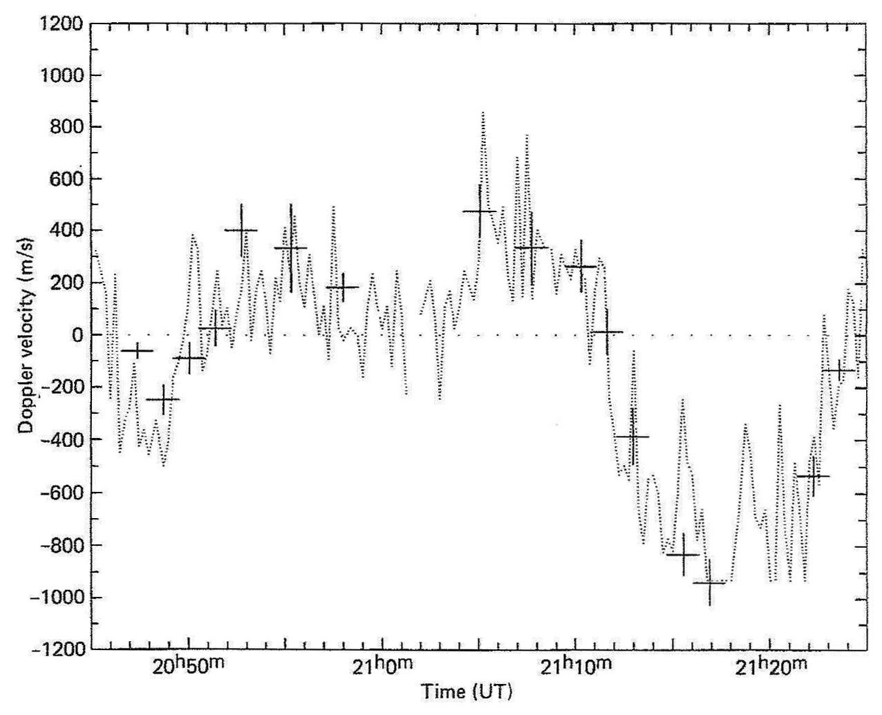
Figure 6 Comparison of plasma drift measurements obtained with the Sondrestrom ISR and irregularity drift measurements obtained with the Goose Bay HF Radar. The radars were looking toward each other, so the sign of the Goose Bay measurement has been reversed. Details of this comparison are given in the text and in Ruohoniemi et al. (1987). In brief, the dotted line shows Sondrestrom Doppler measurements, with 15 s integration time, while the crosses show the average Goose Bay Doppler velocity measured on beams 10 and 11. Goose Bay values are only plotted if acceptable data were obtained on both beams. The timing errors on the crosses are assumed to be 10 s, which is the time interval that the radar is dwelling on beams 10 and 11. Note that the width of the timing error bars has been enhanced by a factor of 10. Reproduced from Fig. 9 of Ruohoniemi et al. (1987).

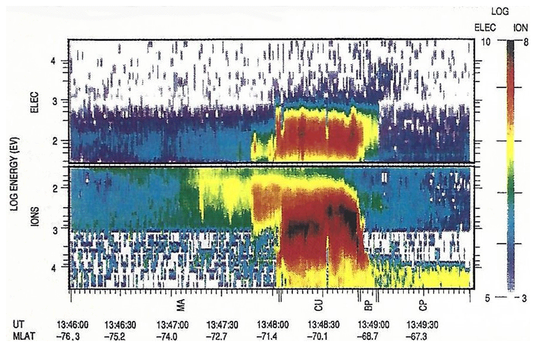
Figure 7 Energy–time spectrograms of electrons and ions obtained on 10 October 1988 by the Defense Meteorological Satellite Program (DMSP) F9 spacecraft. The large ticks on the time axis bound the magnetospheric regions that are associated with the particle spectra that were observed. These regions are as follows: MA – mantle; CU – cusp; BP – boundary plasma layer; CP – central plasma sheet. Note that the spacecraft was detecting the cusp from 13:48:05–13:48:54 UTC (universal coordinated time). Reproduced from Fig. 1b of Baker et al. (1990).

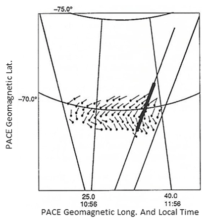
Figure 8 A two-dimensional plot of plasma convection over Antarctica, as observed with the Halley HF Radar. Each dot in the figure indicates the latitude and local time of the measurement, and the length and direction of each line represents the magnitude and direction of the velocity. Note that south is at the top of the figure and west is to the right. The line extending from the bottom upwards toward the right, and superimposed by a bold line, is the trajectory of the DMSP spacecraft. The bold line represents the interval at which it is detecting the cusp plasma shown in the previous figure. Reproduced from Fig. 2 of Baker et al. (1990). Note: MLT – magnetic local time.

3 Additional HF radars in North America and Antarctica

Even while the upgrades to the Goose Bay radar were being completed, funding for additional HF radars in North America and Antarctica was becoming available. Dr Christian Hanuise of the Université de Toulon obtained financial support in France to redeploy his SAFARI electronics from Sweden to the McGill University Sub-Arctic Research Station in Schefferville, Quebec, Canada. He also purchased eight log-periodic antennas and towers from Sabre Communications. The antenna array was installed at Schefferville in the summer of 1986, and joint operations with Goose Bay began in October. Initially, the Schefferville radar did not have a phasing matrix, but a beam was formed by combining the received signals from all eight antennas. This beam intersects half of the beams of the Goose Bay radar (See Fig. 3). During each Goose Bay scan, the Schefferville radar made soundings of the ionosphere at eight frequencies between 8 and 18 MHz.

The Antarctic radar was funded jointly by the British Antarctic Survey and the NSF Office of Polar Programs. The principal investigators (PIs) on this Project were Ray Greenwald of JHU/APL and John Dudeney of the British Antarctic Survey (BAS). Mike Pinnock (BAS) and Kile Baker (JHU/APL) were identified as co-investigators. Under the terms of an agreement between the PIs, JHU/APL would provide BAS with 16 HF log-periodic antennas, two microcomputers, one digital tape drive, disk drives and interface cards, a frequency synthesizer, power supplies, printed circuit boards and component parts for the HF radar transmitters, receiver, phasing matrix, high-power and low-power $T/R$ switches, and other switches used in the phasing matrix. Finally, Kile Baker would accompany our British colleagues on the trip to Antarctica and participate in the construction effort. On their side, BAS would be responsible for the construction of the radar in Antarctica, all future maintenance costs, the development of data display software associated with the Halley radar, and costs for tapes and other recording media required for the Halley data. Copies of the data would be sent to JHU/APL. Both BAS and JHU/APL agreed to fully share their respective data sets and jointly plan special operations.

This project between BAS and JHU/APL was identified as the Polar Anglo-American Conjugate Experiment (PACE), and its objective was to obtain a better understanding of ionospheric processes occurring in the ionosphere at opposite ends of geomagnetic field lines. Figure 4 shows a polar projection of the Northern Hemisphere, including the field of view of the Goose Bay radar. Superimposed on this map is a magnetically conjugate map of Antarctica and the location and field of view of the proposed PACE radar at Halley Station, Antarctica. The common viewing area of the two radars is quite large and represents a significant fraction of the land area of Greenland.

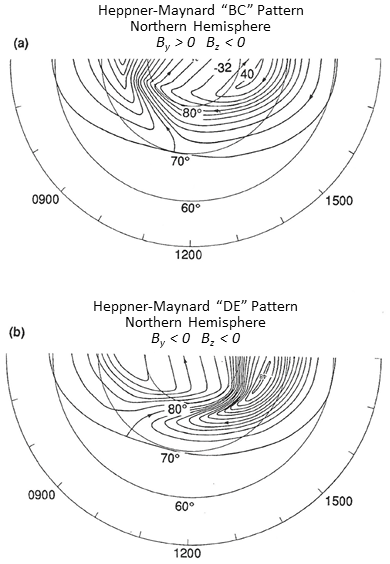
Figure 9 Dayside portions of convection maps obtained by Heppner and Maynard (1987), using data from the Dynamics Explorer (DE-2) spacecraft. The upper pattern (a) is observed in the Northern Hemisphere when IMF B_z is negative and IMF B_y is positive and in the Southern Hemisphere when IMF B_z and IMF B_y are negative. The lower pattern (b) is observed in the Northern Hemisphere when IMF B_z and IMF B_y are negative and in the Southern Hemisphere when IMF B_z is negative and IMF B_y is positive. How quickly do these transitions take place? Reproduced from Fig. 1 of Greenwald et al. (1990).

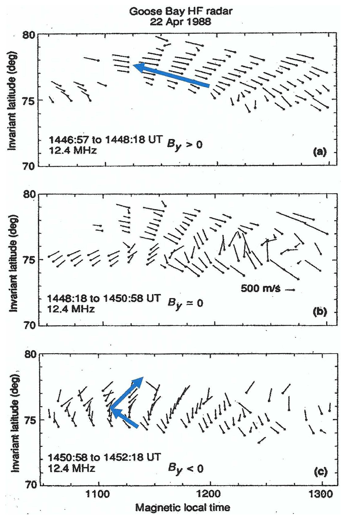
Figure 10 This figure displays how a single HF radar can track the convection dynamics that are associated with a transition in IMF B_y from positive to negative. Panel (a) shows the plasma convection in the vicinity of the cusp just prior to the B_y transition. Most vectors are directed toward the northwest. Panel (b) shows the data obtained by averaging the next two scans. At the highest latitudes, there is still evidence of the B_y positive state, while, at lower latitudes, a new pattern is forming. Finally, in panel (c), a fully formed B_y-negative convection pattern is seen. Blue arrows have been inserted to help the eye. Adapted from Fig. 9 of Greenwald et al. (1990).

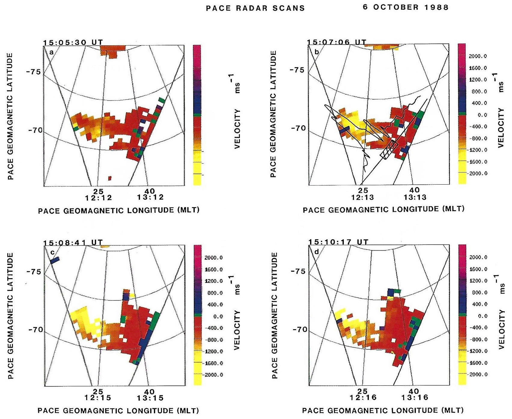
Figure 11 On 6 October 1988, the Halley radar detected six enhanced flow channels in the cusp ionosphere. Of these, one occurred at 15:07–15:08 UTC in association with a passage of the DMSP F7 spacecraft through the Halley radar field of view (see b). The hatched region along the trajectory identified the location of the cusp, and the curved line indicates the drift velocity of the plasma toward the northwest. Reproduced from plate 2 of Pinnock et al. (1993).

The BAS ship, RRS Bransfield, transported the radar electronics, antennas, and towers from the UK to the Falkland Islands, where Dudeney, Baker, Pinnock and Leonard, the PACE radar construction and operations team, boarded the ship. During the remainder of the cruise to Halley, the PACE team began to assemble the antennas and towers. The ship arrived at Halley Bay on 22 December 1987 (1 d after midsummer in the Southern Hemisphere). Over the next 19 d, the PACE team, with support from members of the Bransfield's crew and the Halley site crew, fully assembled the antenna array and installed the radar electronics. First observations were made on 10 January 1988, and routine operations began on 20 January 1988. The Bransfield departed from Halley Bay on 22 January 1988. All members of the PACE construction team, other than Mark Leonard, were aboard the ship. Leonard would remain at Halley for the following 2 years as a site engineer and scientist for the PACE radar.

John Dudeney and Ray Greenwald traveled to Goose Bay in late February 1988 for the first conjugate campaign using the Goose Bay and Halley Bay radars. During this campaign, we had access to the International Maritime Satellite (Inmarsat) communications system, which was developed to support sea-to-shore communications. We had special permission to use this resource to compare conjugate observations of the polar ionosphere. During this campaign, there was a major solar disturbance which disrupted satellite communications and resulted in our being told that the Halley Bay radar was no longer in the ocean sector where it was specified to be located. Such are the impacts of solar disturbances on high-latitude communications.

Figure 5 shows a photograph of John Dudeney standing on the road between our operations building at Goose Bay and the HF radar antenna arrays. Immediately behind him is the main HF antenna array, and further in the background is a portion of the HF interferometer array.

4 Selected results from the pre-SuperDARN HF radars

Over the 6-year period from the start of Goose Bay operations to the end of the decade, HF radar observations from Goose Bay, Schefferville, and Halley produced exciting results over a broad range of topic areas. Here, I describe some of the results that contributed to the creation of the SuperDARN radar network.

4.1 Comparison of irregularity and plasma drifts

The earliest comparison of F-region irregularity and plasma drifts was carried out by Villain et al. (1985) using two SAFARI HF radars and the EISCAT UHF incoherent scatter radar in northern Scandinavia. Those measurements indicated that there was relatively good agreement between F-region irregularity and plasma drifts. A total of 2 years later, Ruohoniemi et al. (1987) reported a similar comparison of HF radar Doppler velocities derived from refined ACFs that were associated with F-region ionospheric irregularities and UHF incoherent scatter observations of plasma Doppler velocities observed with the Sondrestrom radar. For this comparison, the Sondrestrom radar was directed toward Goose Bay, Labrador, at an elevation angle of 30^∘, while the Goose Bay radar performed a 16-beam scan with the direction toward Sondrestrom, which is halfway between Goose Bay beams 10 and 11. (Note that the leftmost beam is beam zero and the rightmost is beam 15.) The Sondrestrom measurements were continuous over the 40 min experiment, with each data point being the result of a 15 s integration, while the Goose Bay radar was scanning and only fixed on beams 10 and 11 for 10 s of each 80 s scan. The common viewing area was approximately 1200 km from Goose Bay and 500 km from Sondrestrom. Figure 6 compares the plasma velocity measured by the Sondrestrom radar (dotted trace) with the average irregularity velocity measured on beams 10 and 11 by the Goose Bay radar (solid crosses). Crosses are plotted only if acceptable measurements were obtained from both beam 10 and beam 11. Note that the signs of the Goose Bay velocities have been negated in this plot to account for the fact that the two radars are looking in opposite directions. Additional details of the nature and geometry of the comparisons are described in Ruohoniemi et al. (1987).

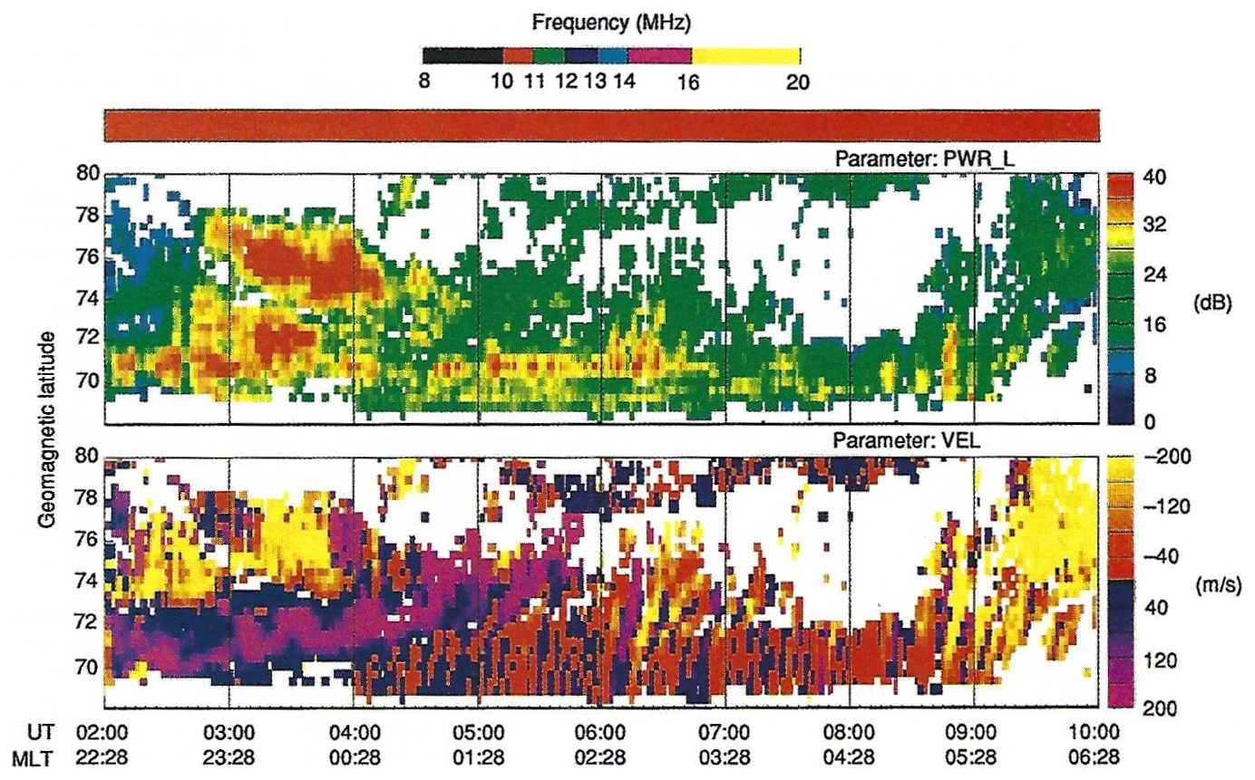
Figure 12 Range–time plot of PWR_L (SNR) and VEL in decibels and meters per second, respectively. The region in the velocity plot from 04:00–09:00 UTC and equatorward of 72^∘ is a long-lasting pulsation event in the post-midnight ionosphere. It is associated with one of the preferred oscillation frequencies first identified by John Samson. Note that the power parameter has an appended L, indicating that it was calculated from the ACF assuming an exponential decay. Both the PWR and width parameters are calculated for both exponential (e^−λt) and Gaussian ($e^{-\mathit{\sigma }{t}^{\mathrm{2}}}$) decorrelations, but in 75 %–90 % of the cases, the exponential decorrelation is most consistent with the observations. Reproduced from plate 2 of Walker et al. (1992).

The 15 s incoherent scatter radar measurements show more variability than the estimated errors associated with the Goose Bay radar measurements. This variability is most likely due to the lower SNRs of incoherent scatter measurements, which introduce more statistical noise. Other plots in Ruohoniemi et al. (1987) use an average of eight (15 s) integrations and do not show large fluctuations. Overall, the two data sets show similar behavior, indicating that F-region irregularities are embedded in the plasma and move at the $(E\times B)/B^{\mathrm{2}}$ drift velocity.

4.2 Ionospheric signatures of dayside magnetospheric reconnection

During the latter years of the 1980s and throughout the 1990s, significant scientific attention was directed toward dayside magnetospheric reconnection, its impacts on plasma circulation in the dayside high-latitude ionosphere, and the entry of solar wind plasma to the inner magnetosphere. In response to this interest, the NSF Geospace Environment Modeling (GEM) program was initiated to identify ionospheric signatures of plasma processes associated with dayside reconnection. When GEM began, the best ionospheric signatures of dayside reconnection in the high-latitude magnetosphere were provided by particle detectors on low-Earth-orbit, high-inclination spacecraft. The most readily available of these were the DMSP series of spacecraft developed under contract from the Air Force Weather Service. Figure 7 shows an example of particle signatures obtained by the DMSP F9 spacecraft as it traversed the field of view of the Halley PACE radar. The figure shows that, in the latitudinal strip from −71 to −69^∘ magnetic latitude, the DMSP spacecraft detected large fluxes of magnetosheath plasma (electrons with energies of ∼ 100 eV and ions with energies of ∼ 1 keV) precipitating into the ionosphere. Newell and Meng (1988) identified electrons and ions with these energies to be characteristic of electrons and ions in the dayside magnetosheath.

Figure 13 Range–time plot of PWR_L in dB and Doppler velocity. Note the equatorward-moving strong intensifications in backscattered power that are associated with low Doppler velocities. These intensifications are due to Earth-reflected atmospheric gravity waves that are produced at high latitudes and propagate equatorward and downward. After being reflected by the Earth, they return to the ionosphere where they create a pattern of southward-moving neutral density enhancements in the ionosphere. These, in turn, create a southward-moving corrugated electron density pattern on the bottomside of the ionosphere. Further details are given in Fig. 14. Reproduced from plate 3 of Samson et al. (1990).

The reconnection process itself, while not fully understood, is thought to involve magnetic field lines in the solar wind contacting geomagnetic field lines at the outer boundary of the magnetosphere. If these field lines are oppositely directed at the point of contact, they can break and reconnect with those portions of the solar wind field line that best retain continuity of the geomagnetic field direction. This condition allows for an exchange of solar wind and magnetosphere and/or ionosphere plasmas, leading to the particle signatures detected by the DMSP spacecraft and the development of plasma turbulence in the reconnection region and along the reconnected field line. The solar wind portion of each reconnected field line drags the newly reconnected magnetic flux tube in an anti-sunward direction. This process is thought to be dynamic and confined to relatively localized and spatially varying regions on the high-latitude, dayside magnetopause. As the magnetic flux tubes are dragged anti-sunward, they migrate toward the central plasma sheet in the Earth's magnetotail. When the flux tubes from the Northern and Southern hemispheres come together, they undergo a second reconnection process, forming distinct geomagnetic and solar wind field lines. The geomagnetic field lines are transported sunward within the magnetosphere, while the solar wind field lines continue to be dragged anti-sunward by the solar wind plasma.

Shortly after the GEM Program began, the DMSP F9 data shown in Fig. 8 were compared with Halley PACE radar observations of plasma convection in the vicinity of the ionospheric footprint of the dayside cusp. Figure 8 shows the 2-D convection pattern derived from two consecutive 80 s scans of the Goose Bay radar. The solid line shows the satellite trajectory, and the superimposed bold line indicates the portion of the trajectory where cusp precipitation was observed in Fig. 8. In the equatorward half of the cusp, the convection velocities are toward the northwest at speeds ranging from 800–1000 m/s, while at the poleward half of the cusp, the velocity vectors had rotated to the northeast, and the speed had increased to 1000–1200 m/s (Baker et al., 1990).

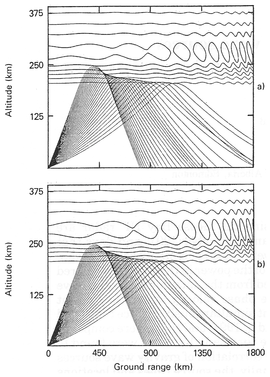
Figure 14 Ray-tracing analysis of radio wave propagation through an ionosphere impacted by an Earth-reflected gravity wave. The corrugated electron density surfaces on the bottom of the ionosphere affect the propagation of transmissions from an obliquely directed HF radar. Where the surfaces are concave relative to a ground observer, the ray paths are altered by reflection and tend to converge as they approach the Earth's surface, leading to stronger backscattered signals. In contrast, rays that are incident on convex surfaces in the bottomside ionosphere are dispersed upon reflection, leading to weaker forward power and weaker backscatter. Panel (a) in this figure shows the backscatter distribution 195 min after the gravity wave was generated. Bunches of incoming rays are observed at ground ranges of 1300 and 1800 km. Panel (b) shows the backscatter distribution at 210 min after gravity wave excitation. The bunches of incoming rays have moved toward the radar-to-ground ranges of 1100 and 1600 km. Reproduced from Fig. 2 of Samson et al. (1990).

4.3 Conjugate observations of convection near the cusp

Historically, large-scale maps of plasma convection patterns or electrical potential patterns in the high-latitude ionosphere and outer magnetosphere were obtained from satellite measurements of electric fields or plasma drift. These studies required large databases not only of the measurements but also of supporting parameters, such as the magnitude and orientation of the interplanetary magnetic field (IMF) and the speed and density of the solar wind. Large data sets were required because high-inclination satellites often have orbits that precess very slowly in local time. It could take months to years to acquire enough measurements to extract meaningful global convection or potential patterns. Since the patterns are very dependent on the properties of the solar wind and the magnitude and direction of the IMF, care must be exercised to assure that only data sets that were obtained within limited ranges of IMF B_x, B_y, and B_z, solar wind speed, and solar wind density are used in any specific analysis. Figure 9 displays a pair of convection patterns obtained by Heppner and Maynard (1987). These authors found that if IMF B_y was positive and IMF B_z was negative, dayside plasma convection in the Northern Hemisphere would resemble panel (a), whereas if IMF B_y and IMF B_z were both negative, dayside convection would resemble panel (b). These authors also found that the same patterns could be observed in the southern polar region, under IMF B_z negative conditions, but the sign of IMF B_y was reversed. That is, for IMF B_y positive conditions the convection panel in the Northern Hemisphere appears as it does in the upper panel of Fig. 9, and the convection pattern in the Southern Hemisphere appears as it does in the bottom panel. If IMF B_y is negative, the Northern Hemisphere would display the bottom panel and Southern Hemisphere would display the top panel.

In the case of radar measurements, the situation is somewhat different. If we are interested in global patterns, we may still need to retain a database of solar wind and IMF parameters, but if we are only interested in more mesoscale aspects of the convection patterns, we may find that we only need to obtain the IMF and solar wind parameters for a single interval.

Greenwald et al. (1990) used the PACE radars to examine conjugate patterns of convection near the cusp and the evolution of the convection pattern during a period in which IMF B_z remained negative while IMF B_y made several transitions between positive and negative. In this paper, there are several examples in which convection in the Northern Hemisphere was either consistent with IMF B_y positive or negative, while the Southern Hemisphere convection pattern was always in the complementary state. However, the most interesting result of this paper is shown in Fig. 10. Figure 10a shows the convection pattern observed in the Northern Hemisphere with the Goose Bay radar. Each of the measurements in this figure is indicated by a dot, locating its invariant latitude and local time, and a line extending from the dot, showing the direction and magnitude of the drift velocity. The convection pattern in Fig. 10a is in a west-northwestward direction and IMF B_y is positive. The scale indicated in Fig. 10b can be used to estimate the drift speeds in all three panels. Most of the drift speeds range from 800 to 1600 m per second. These convection patterns extend over 7–10^∘ in invariant latitude and ∼ 3 h of magnetic local time. In Fig. 10b, the effects of a transition to IMF B_y negative are beginning to be observed. Poleward of 76^∘ invariant latitude, we still observe west-northwestward convection, but at lower latitudes the convection is rotating toward the northeast. Finally, in Fig. 10c, the clockwise rotation of the dusk convection cell has expanded poleward to fill the field of view. This is the dominant convection that would be expected near noon for an IMF B_y negative condition. The total time for this transition to completely fill the field of view of the Goose Bay radar is somewhere between 2 and 3 min. The ability of PACE radars to measure convection changes over large spatial areas in relatively short periods of time is clearly an important capability for understanding plasma processes that couple the solar wind, magnetosphere, and ionosphere.

4.4 Transient convection enhancements near the cusp

In the early 1990s, Mike Pinnock and coworkers identified periods of transient ionospheric flow enhancement near local noon in the field of view of the Halley radar. Pinnock et al. (1991) reported one example of transient, longitudinally extended enhanced convection near the cusp but did not have associated satellite data. More recently, Pinnock et al. (1993) identified other examples of transient convection channels within the cusp. In these cases, there were supporting data from the DMSP F9 spacecraft that included drift meter observations (see Fig. 11). On the 15:07 UTC scan of the radar, both the drift meter and the Halley radar observed convection velocities of 2–3 km per second, while the hatched area along the trajectory indicates where cusp precipitation was observed. The spacecraft passed across the convection channel, only observing it for ∼ 20 s, whereas the Halley radar observed the same flow channel for several minutes. On this day, the Halley radar observed eight transient flow channels between 14:29 and 15:31 UTC. These channels were separated by 4–7 min and had lifetimes of 3–4 min. When enhanced flow channels were active, the convection velocities exceeded 2000 m per second.

4.5 Geomagnetic pulsations in the Earth's magnetosphere and ionosphere

Geomagnetic pulsations are large-scale oscillations of geomagnetic field lines that are generally footed in the mid- to high-latitude ionospheres in both hemispheres. They are excited by pressure and magnetic field disturbances in the solar wind and by plasma disturbances in the magnetotail. The signatures of geomagnetic pulsations were observed with radars for many years, but the interpretation of these observations awaited the construction of the STARE VHF radars in northern Scandinavia and the work of Walker et al. (1979). STARE measurements were limited to $\mathrm{65}{}^{\circ }\le \mathrm{\Lambda }\le \mathrm{69}{}^{\circ }$, whereas the Goose Bay radar can obtain measurements from $\mathrm{64}{}^{\circ }\le \mathrm{\Lambda }\le \mathrm{80}{}^{\circ }$. This allows the Goose Bay radar to detect a wider range of pulsation frequencies and, potentially, to detect pulsation phenomena in more remote regions of the Earth's magnetosphere.

Dave Walker of the University of KwaZulu-Natal, South Africa, and John Samson of the University of Alberta, Canada, worked with some of the early data from the Goose Bay radar, particularly data relating to pulsations detected at higher geomagnetic latitudes. Figure 12 is a figure from Walker et al. (1992), showing an example of Goose Bay data in range–time–parameter format. The lower panel in the figure shows a time series of Doppler velocities observed on beam 6 of the Goose Bay radar between 02:00 and 10:00 UTC. The Doppler velocities observed from 04:00 to 09:00 UTC at geomagnetic latitudes between 69 and 72^∘ are associated with pulsations. These Doppler velocities are being driven by an oscillating electric field in the overhead ionosphere, and the magnetic field line that is oscillating most strongly is in resonance with a driven oscillation that may be propagating tailward along the magnetopause. An interesting point concerning both the STARE and Goose Bay data is that there appear to be preferred frequencies (in millihertz) for these oscillations (∼ 0.8, 1.3, 1.9, 2.6, and 3.4 mHz). Ruohoniemi et al. (1991) presented observations made with the Goose Bay radar, showing examples of two of these preferred oscillation frequencies and how they transitioned from one frequency to the other. John Samson identified the preferred frequencies as being associated with cavity modes (Samson et al., 1991, 1992); while Walker et al. (1992) preferred to associate them with waveguide modes. In the end, these authors concluded that the four higher of these preferred frequencies were best described as waveguide modes but noted that it was not likely that the ∼ 0.8 mHz oscillation could easily fit into that description (Samson et al., 1992).

4.6 Atmospheric gravity waves

On an earlier sabbatical visit to JHU/APL, John Samson was also attracted to another research topic that was outside his main interests. This research topic was atmospheric gravity waves and their impact on HF radar backscatter. Atmospheric gravity waves are neutral disturbances in the upper atmosphere that propagate at acoustic velocities in the upper atmosphere and distort the iso-density contours of the ionized component of the ionosphere. Figure 13 displays range–time–parameter plots of SNR and Doppler velocity for a gravity wave event observed with the Goose Bay radar (Samson et al., 1990). Note that in the period from 13:30–20:00 UTC, there are enhancements in the backscattered power that propagate equatorward for up to 2000 km. Since we are looking at ground backscatter, the actual range of the ionospheric reflection point is one-half of the range associated with the ground reflections shown in Fig. 13.

John Samson searched the gravity wave literature and identified a paper by Francis (1974) that discussed the evolution of a current impulse in the upper E layer of the ionosphere. This impulse would transfer energy and momentum to the surrounding neutral atmosphere, and this perturbation to the neutral atmosphere would travel outwards both horizontally and obliquely downwards. While it would be totally undetectable as it approaches the Earth's surface, upon reflection it would propagate upward and grow relative to the background neutral atmosphere. When the reflected gravity wave reaches ionospheric heights, the neutral density perturbation would impact the electron density profiles in the manner shown in Fig. 14. Note that, where the electron density contours are concave relative to the ground, the reflected rays of the radar signals are focused more closely together, intensifying the backscattered signals. This is to be contrasted with regions where the electron density contours present a convex face to the ground, and the reflected rays are dispersed, resulting in backscattered powers that are very much weaker or unobservable.

The top and bottom panels in Fig. 14 represent the electron density contours 195 and 210 min after gravity wave excitation. In the 15 min between these panels, the focusing that was occurring near 1900 km has moved to a ground range of 1600 km. If we traced the intensity enhancements in Fig. 14 back to a common origin, we would find that the gravity wave resulted from a shear flow enhancement 2250 km poleward of the Goose Bay radar at 12:15 UTC. In fact, this current surge occurred near the ionospheric footprint of the cusp.

5 Summary

It is hoped that this post-1980 history of HF radar research in the USA, Canada, and Antarctica has provided the reader with some appreciation of the complexities that are associated with HF radar measurements in the ionosphere and, also, a greater appreciation of the potential that these measurements have for advancing our understanding of plasma processes in the Earth's very high latitude ionosphere and outer magnetosphere. From the beginning, the objectives were to investigate physical processes that occur over large regions of the high-latitude ionosphere and to encourage the participation of others who might share in this vision.

An item I have not mentioned is that, in 1979, NASA released an Announcement of Opportunity for a four satellite mission known as Origin of Plasmas in the Earth's Neighborhood (OPEN). In addition to the spacecraft investigation teams, funding was made available for four ground-based investigation teams and four theory teams who would also support this mission. I submitted a proposal entitled Dual Auroral Radar Network (DARN) for this mission and BAS, as an organization, also submitted a proposal entitled Satellite Experiments Simultaneous with Antarctic Measurements (SESAME). Both proposals were selected as part of the ground-based segment of this mission. There were, however, some caveats. First, the radars in the DARN proposal were E-region radars of the STARE type, and secondly, NASA was not prepared to put any funding into the development of ground-based experiments. A decade later, as the situation evolved, my BAS colleagues and I were pleased with the results we were obtaining from the PACE radars and the four remote, automatic geophysical observatories that BAS had deployed. The only thing that would have been better would have been to expand the network of HF radars in the high-latitude regions of both the Northern and Southern hemispheres. Essentially, our goal was to turn DARN into SuperDARN. The next portion of this history will describe how this deployment evolved into the early years of the 21st Century.