At the dawn of global climate modeling: the strange case of the Leith atmosphere model

A critical stage in the development of our ability to model and project climate change occurred in the late 1950s–early 1960s when the first primitive-equation atmospheric general circulation models (AGCMs) were created. A rather idiosyncratic project to develop an AGCM was conducted virtually alone by Cecil E. Leith starting near the end of the 1950s. The Leith atmospheric model (LAM) appears to have been the first primitive-equation AGCM with a hydrological cycle and the first with a vertical resolution extending above the tropopause. It was certainly the first AGCM with a diurnal cycle, the first with prognostic clouds, and the first to be used as the basis for computer animations of the results. The LAM project was abandoned in approximately 1965, and it left almost no trace in the journal literature. Remarkably, the recent internet posting of a half-century-old computer animation of LAM-simulated fields represents the first significant “publication” of results from this model. This paper summarizes what is known about the history of the LAM based on the limited published articles and reports as well as transcripts of interviews with Leith and others conducted in the 1990s and later.

1 The beginnings of comprehensive numerical climate modeling

Today, the numerical modeling of the global climate is an enterprise employing many hundreds of scientists and support staff working at dozens of institutions, and the results of contemporary global climate models inform some of the world's most consequential public policy decisions. By contrast, the crucial pioneering efforts on global atmospheric modeling in the 1950s and early 1960s were conducted by less than a handful of remarkably small groups. The notion of numerical time integration of the governing equations was initially developed in the context of short-term weather forecasting in the visionary work of Richardson (1922) and then in the more practical approaches of Charney et al. (1950) among others. Phillips (1956) performed the first numerical experiment designed to understand the global circulation of the atmosphere using an extended simulation from arbitrary initial conditions. The study by Phillips (1956) employed a model with simplified geometry (replacing the globe with a plane) and dynamics (a crude two-level discretization of the quasi-geostrophic equations) as well as a very crude representation of radiative heating and cooling. The success of the abovementioned study naturally led to a desire for similar experiments with models that included more realistic aspects of the atmosphere, notably adopting the primitive equations and incorporating physically based treatments of the radiative heating/cooling as well as the basic processes in the hydrological cycle.

The earliest effort developing a global primitive-equation model was led by Joseph Smagorinsky at the General Circulation Research Section of the US National Weather Service (the forerunner of today's Geophysical Fluid Dynamics Laboratory, GFDL) starting in 1956 (Smagorinsky, 1983). This produced classic papers on the original versions of the model (Smagorinsky, 1963; Smagorinsky et al., 1965) and was the basis for the later development of many influential climate models at the GFDL (Edwards, 2000). Another pioneering modeling effort was led by Akio Arakawa and Yale Mintz at the University of California Los Angeles (UCLA) who began work on a two-level primitive-equation global model in 1961 with a version including a hydrological cycle completed in the middle of 1963 (Johnson and Arakawa, 1996; Edwards, 2000). This model was then further developed at UCLA and elsewhere, resulting in a “family” of UCLA-related global models (Arakawa, 2000; Edwards, 2000); at least one “direct descendent” is a UCLA climate model that is still used today (e.g., Kang et al., 2019). In 1964, another major effort was begun to develop global circulation models at the National Center for Atmospheric Research (NCAR). From this beginning (Washington and Kasahara, 1967; Edwards, 2000), NCAR developed a major and ongoing climate modeling enterprise.

While the well-known GFDL, UCLA, and NCAR pioneering models all led directly to continuing high-profile climate modeling activities at each of the three centers, there was a fourth AGCM project that began around 1958 which produced results that aroused interest at the time but did not lead directly to an ongoing climate modeling effort that still continues today. This was essentially a one-person effort by Leith at the Lawrence Radiation Laboratory, and the model that resulted was referred to as the LAM – which may stand for either the “Leith atmosphere model” or the “Livermore atmosphere model” (Edwards, 1997). In this paper, I will trace the unusual story of the LAM which is now virtually unknown among the climate modeling community.

2 Cecil E. Leith and his pioneering atmospheric modeling effort

Cecil E. “Chuck” Leith (1923–2016; Fig. 1) earned his undergraduate and PhD degrees in mathematics at the University of California Berkeley. In World War II he worked on the Manhattan Project to develop the first nuclear weapon. In 1946 he joined the Lawrence Radiation Laboratory (LRL; later the Lawrence Livermore Radiation Laboratory that became today's Lawrence Livermore National Laboratory, LLNL) and developed numerical simulations of nuclear explosions which, as he himself noted, involved “hydrodynamics and radiation transport and neutron transport…” (Edwards, 1997). Around 1958 Leith began to consider the development of a global atmospheric circulation model as a major activity, and in 1960 he produced the first version of the LAM. In the mid-1960s he presumably realized the limitations of explicit global simulations of moderate resolution and the central importance of parameterizing the subgrid-scale effects of large-scale turbulence on the resolved flow in atmospheric models and changed his focus to turbulence theory (Leith, 1968a, b, 1969) and later to atmospheric predictability and related topics (Leith, 1971), which were areas that he pursued for the next 3 decades (Leith, 1988). In the first half of his career, Leith published almost nothing, presumably due to the classified nature of his early work and then due to whatever inhibited him from writing up his LAM results in the early 1960s (Michael MacCracken, personal communication, 2020, suggests two possible reasons: the absence of a culture at LRL that valued journal publication, and the difficulty in producing publication-quality graphics). Once he focused on turbulence theory, Leith became a prolific author and published many influential papers.

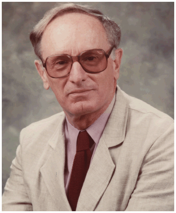
Figure 1 Photo of Cecil E. “Chuck” Leith. From Zhou and Herring (2017).

A 2017 special issue of the journal “Computers and Fluids” honored Leith's scientific contributions to fluid mechanics. It is interesting that none of the 15 contributions to the issue were devoted to global atmospheric modeling, and the introductory essay by Zhou and Herring (2017) makes only a passing reference to the general circulation model development phase of Leith's career.

In 1968, Leith joined NCAR, where he stayed until 1983, before returning to LRL for the remainder of his career. He was the director of NCAR's Climate Division from 1978 until 1982. It seems he never pursued the LAM model at NCAR, and while he presumably encouraged the climate model development effort at NCAR, he was never directly involved.

3 Sources for the history of the LAM

The first inkling I had of the existence of the LAM occurred when I read Hunt and Manabe (1968) which is the first journal article to report on the simulated diurnal cycle and atmospheric tides in an AGCM. In their summary of the very limited previous work in this area, Hunt and Manabe (1968) stated the following:

Atmospheric tides have been obtained previously with [comprehensive AGCMs] by Mintz [reference to a 1965 World Meteorological Organization report] and Leith. Mintz computed a semidiurnal tide at the Equator of 1 mb amplitude… using a two-level model with a highly parameterized scheme for computing the radiative heating. Leith also obtained a semidiurnal oscillation with another general circulation model, in which the radiative heating due to the absorption of insolation by water vapor was calculated, but has only “published” his results in the form of a short, but beautifully made, documentary film.

(It is clear that by “documentary film” they were referring to what today we would call a “computer animation”.)

This appears to be the only mention of Leith's model results in the near-contemporaneous journal literature. A description of the formulation of the model (but without any results or even an indication that the code had been successfully run on a computer) was published by Leith in 1965 in a chapter in one of a series of books entitled “Methods in Computational Physics” (Leith, 1965a). Another brief treatment of the issues involved in the formulation of the LAM appeared in an agency progress report (Leith, 1966) which is almost identical to a paper in an American Mathematical Society conference proceedings (Leith, 1967). A brief paper by Leith also appeared in a mixed Russian and English language conference proceedings volume that was edited, published, and printed in the Soviet Union (Leith, 1965b). This seems to be the only publication by Leith showing a (tiny) glimpse of actual results of the LAM model integrations – in this case a single Northern Hemisphere (NH) map of instantaneous surface pressure and precipitation, as well as height–latitude sections of the “typical distribution of energy sources and sinks”. Unfortunately, the figures, particularly for the energy sources and sinks, are nearly illegible, and it is impossible to decipher what the contour values are or even what exact quantities are plotted in each panel. Oddly, these published results are from a version of the model testing an experimental moist convection parameterization that led to quite unrealistic results compared with the more successful model version using a simpler treatment of the moist processes described in Leith (1965a). Finally, Hardy (1968) discusses an analysis of the solar tidal signals in a LAM simulation in an internal LRL report.

The discussion of the development of the model in the next section also makes use of transcripts of two interviews that Leith gave in the 1990s, one focused on his contributions to atmospheric modeling (Edwards, 1997) and one that ranged more widely over his entire career (Michael, 1994). Leith gave a talk in 2002 at a 50th anniversary celebration for LLNL. A video of his talk was very recently made available online at https://youtu.be/f96Q8AdKhpQ (last access: 20 April 2020). Some insight into the reception of Leith's efforts and later developments related to Leith's model are provided in transcripts of interviews given by NCAR's Warren Washington (Edwards, 1998) and LLNL's Michael MacCracken (Hundebol, 2013). A brief discussion of the LAM is included in a recent LLNL perspective on current climate modeling issues (Linehan, 2017), and the LAM is also very briefly discussed in the recent review paper of Randall et al. (2019). MacCracken, who was Leith's graduate student circa 1964–1968 and wrote his PhD thesis on the development and application of a two-dimensional version of LAM, provided his valuable reminiscences directly to the author (referenced here as “Michael MacCracken, personal communication, 2020”).

4 The development of the LAM

Leith's account in Edwards (1997) shows that he began to seriously contemplate applying his computational physics expertise to the problem of atmospheric simulation in the late 1950s. This interest was encouraged by the LRL director at the time, the famous nuclear physicist Edward Teller. Leith (1988) states the following:

It was in the late 1950's that Edward Teller encouraged me to investigate the role that newly available computing power at Livermore might play in achieving a more complete numerical simulation of the global atmosphere. This led to the construction of the first atmospheric model with an explicitly computed cycle of water vapor evaporation, transport and condensation.

Leith at this point had established a substantial reputation within the LRL and had been given a kind of sabbatical to investigate possible new research topics (Michael MacCracken, personal communication, 2020). In his interviews (Michael, 1994; Edwards, 1997) and his 2002 talk at LLNL, Leith pretty clearly implied that he was essentially a free agent and was looking for a challenging research area. In his 2002 lecture, Leith noted an important motivation for taking up the problem of atmospheric numerical simulation at the end of the 1950s was finding an outlet for his interests and expertise in hydrodynamics as he perceived that nuclear weapons research might be curtailed with the increasing likelihood of nuclear test bans (which did ultimately materialize beginning with the Limited Nuclear Test Ban treaty of 1963). In his 1997 interview, Leith explained the following:

When I got interested in it, I talked to [Teller] about it, and he was very supportive of my going into this. He had known about the stuff going on at Princeton [i.e. Charney's work on numerical weather prediction]… he… encouraged me very strongly to start looking into these weather modeling problems.

Leith does not explain the nature of Teller's interest in atmospheric modeling, but Teller already had an interest in climate change – he had presented a talk on carbon-dioxide-driven global warming at an American Chemical Society meeting in 1957 (Matthews, 1959).

In his interview reported in Michael (1994), Leith indicates that his plans and activities for atmospheric modeling were bound up with the expected arrival of a new computer in fall 1960: the Livermore Automatic Research Calculator (LARC), which was the first transistorized computer at LRL. Leith explained his work on this project:

So I pointed out to the people I talked to that I didn't know very much about the atmosphere, but we were about to get a computer that was ten times faster – so didn't it make sense for me to try to build an atmospheric model… I was strongly encouraged to go ahead… I spent about a year or so before the delivery of the LARC in October 1960 – getting ready for it. In fact, during the summer of 1960, I spent some months at the International Institute for Meteorology in Stockholm working on the development of this model code and having access to a library and people who had some familiarity with the nature of the problems encountered in doing this sort of thing. In the fall, I returned to Livermore, the LARC was delivered, and I started running on it. In fact, I think I was running on it quite a bit sooner than almost anyone else, because I had spent this time getting ready for it.

The implication here is that Leith had a version of LAM successfully running in late 1960. Remarkably, the model was written in assembly language, and in his 1997 interview Leith noted that he got a big jump on other users because they were waiting for a compiler to be implemented on the LARC (Edwards, 1997). Later, a FORTRAN version was written which served as the basis for further developments.

In his 1997 interview, Leith recalls that this first version of LAM had five vertical levels and a 5^∘ latitude–longitude grid. The domain was from the Equator to 60^∘ N and free-slip zonal walls were assumed at the Equator and 60^∘ N. The simplified northern boundary was described by Leith as his “quick, initial solution” to the complications introduced by the convergence of meridians near the pole for a latitude–longitude grid. It seems that the major later developments (as described in Leith, 1965a) in the LAM included the construction of a grid that allowed the model to stretch to the pole and the implementation of a six-level vertical structure. Figure 2 shows the six-level vertical structure that was staggered with winds and geopotentials computed on “odd” levels and the temperature, vertical velocity, and water vapor mixing ratio computed on “even” levels. The top level for winds and geopotentials was 50 hPa. In addition, the surface pressure was computed at each time step. The horizontal grid was also staggered with horizontal winds computed on “odd” grid points, whereas temperature and geopotential were computed on “even” grid points.

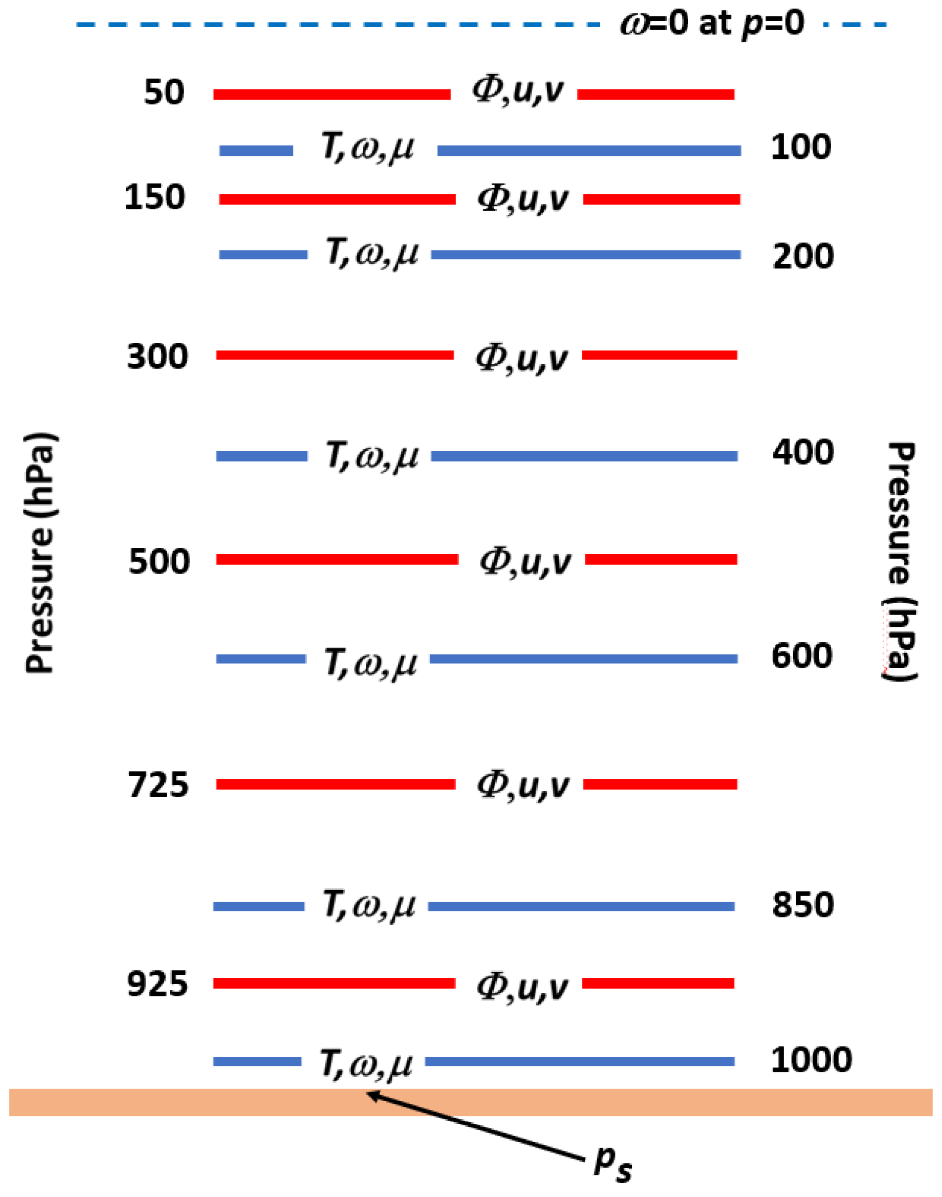
Figure 2 Vertical level structure in the six-level LAM. The variables attached to each level are shown, including the geopotential (φ), the zonal wind (u), the meridional wind (v), the vertical wind in pressure coordinates (ω), the temperature (T), and the water vapor mixing ratio (μ). The surface pressure is also computed.

The model had no topography but included a realistic land–sea distribution. Over the ocean, the surface temperature was specified and the water vapor was assumed to be saturated at the surface. Over “arid land”, the surface temperature was also specified, but the surface mixing ratio was taken to be zero. Standard drag law formulations were used to compute the fluxes of horizontal momentum, heat, and water vapor between the surface and the lowest model level. Horizontal momentum, heat, and water vapor were also transported among levels via a parameterized vertical eddy diffusion.

The heating by water vapor absorption of solar radiation was calculated as a function of the solar zenith angle and the distribution of water vapor mixing ratios in the column. This allowed somewhat realistic shortwave heating rates to be computed, although absorption by other constituents (ozone, carbon dioxide, and aerosols) was ignored in this version. Notably, this formulation should produce a reasonable diurnal cycle of heating in the troposphere. The longwave radiation was treated in an extremely simplified manner, basically specifying a radiative cooling that was just a function of height, with the specified cooling peaking at ∼2.5 ^∘C d⁻¹ at 400 hPa and becoming very small by 100 hPa (for comparison see, for example, the detailed radiation calculations of Manabe and Strickler, 1964, and Dopplick, 1972).

At the end of each time step, an adjustment was made at any point with predicted supersaturation of water vapor assuming that the excess water vapor condenses out and falls to the ground instantaneously as precipitation. Details are lacking in Leith (1965a); however, it is clear that some measure of cloud cover was also predicted in this version of the LAM, but that it did not affect the radiative calculations. Leith (1965b) describes an experimental version of LAM with more sophisticated treatment of hydrological processes and clouds, but he notes that, when the model was run with this moist convective parameterization, the simulated precipitation field became very unrealistic.

The numerical schemes and subgrid-scale parameterizations in the LAM are described in some detail in Leith (1965a) but without any indication that the model code had actually run on a computer. The lack of any actual documented report of a model run leaves some basic questions unanswered such as whether the model was always run with global domain (as opposed to a hemispheric domain with a free-slip Equator). There was also no discussion regarding what specified surface temperatures were used.

So far, we see that the Leith model existed in two initial versions that I will label Version 1 (five levels, 0–60^∘ N domain) and Version 2 (six levels, global domain). It is clear, however, that substantial further development took place beyond the Version 2 (i.e., the version documented in Leith, 1965a), and that we can tentatively identify two further versions (3 and 4). Version 3 is not really documented, but we know that the physical parameterizations had been upgraded by the time that (then graduate student) MacCracken began working with the model. Michael MacCracken (personal communication, 2020) recalls that this version had explicitly calculated longwave radiation as well as predicted radiatively active clouds and included the radiative effect of a prescribed ozone. We can further identify a Version 4 that is documented (incompletely) in Leith (1965b), which was like Version 3 but with an attempt at a more sophisticated moist convection parameterization (which unfortunately was not very successful).

The LAM project eventually entrained efforts from graduate students in the University of California Davis (UCD) Department of Applied Science – an academic department described by Leith as “a kind of Livermore branch” of UCD (Edwards, 1997). In particular, a two-dimensional (zonally averaged) version was developed by MacCracken and applied by him and others to various problems, a story which is briefly summarized at the end of the next section.

5 Was LAM the first comprehensive atmospheric simulation model?

Leith (1988) makes an explicit claim that his LAM was the first simulation model to include a representation of the hydrological cycle (a claim repeated in his 2002 LLNL lecture). This key feature, along with the six-level vertical structure and the use of prognostic water vapor in the radiation calculation, would make it reasonable to consider LAM as the first modern comprehensive atmospheric general circulation model – despite significant simplifications (notably the lack of topography as well as the specified temperature and humidity at the land surface). Of course, by Version 3 of LAM that MacCracken took over circa 1964, the LAM had prognostic, radiatively active clouds – a feature that was not included in other GCMs for at least another decade (e.g., Wetherald and Manabe, 1980).

Unraveling the exact chronology of the developments in the earliest global atmospheric modeling projects is complicated by a culture among the leaders that seems to have permitted very slow publication of results. I have already noted Leith's almost total lack of publications related to LAM – the first not appearing until 1965 (5 years after the initial successful integrations of the model). Smagorinsky (1958) describes the numerical schemes to integrate a two-level, dry, primitive-equation model in a domain bounded by two rigid zonal walls on a spherical Earth. That paper does not present any results but implies that an actual code had been constructed and had run stably. Indeed, Smagorinsky (1983) states that by 1958 the results from a near-hemispheric two-level dry model were complete enough that they could be presented at conferences. Smagorinsky (1983) recalls the following:

The long lapse between this stage and the final publication in 1963 was the result of a personal desire to perform thorough analyses of the non-geostrophic modes and of the energetics. In retrospect, it was a mark of immaturity that I decided not to publish the results in several intermediate stages but rather at the end as a comprehensive work.

How soon the hydrological cycle and the nine-level vertical structure as reported in Smagorinsky et al. (1965) and Manabe et al. (1965) were first successfully incorporated into the GFDL model is not clear. However, there are some indications in the available literature that this very likely occurred well after the end of 1960 when the LAM was presumably already running. Smagorinsky gave a paper at the 12th IUGG General Assembly in Helsinki in July 1960, presenting only results from various experiments with the two-level dry model (Smagorinsky, 1960). Smagorinsky (1983) notes that for the November 1960 International Symposium on Numerical Weather Prediction in Tokyo he presented results of 24 short-term forecasts using a dry, no-topography, frictionless, three-level version of his model. In March 1963 Smagorinsky gave the Symons Lecture of the Royal Meteorological Society on the subject “Some Aspects of the General Circulation”. The written version of his lecture (Smagorinsky, 1964) discusses only two-level dry models. The abstract of a talk authored by Joseph Smagorinsky and Syukuro Manabe presented at an American Meteorological Society (AMS) meeting in New York in January 1963 describes the formulation of a nine-level model like that eventually published in Smagorinsky et al. (1965), although without an indication that any integrations had been performed (see Smagorinsky and Manabe, 1962).

Of course, both the LAM and the GFDL model described in Smagorinsky et al. (1965) had significant limitations that are generally avoided in contemporary models classed as AGCMs. Notably, both models had no topography. In addition, the LAM lacked a treatment of the surface heat balance over land. However, the LAM included realistic features not treated even in the GFDL model of 1965 (and actually not included in GFDL models until several years later); notably, the LAM included diurnal and seasonal variations of the radiation and a prognostic cloud cover scheme.

The LAM code was later used as the basis for a two-dimensional (zonally averaged) atmospheric model that was developed and applied by MacCracken in his PhD thesis at the UCD entitled “Ice Age Theory Analysis by Computer Model Simulation”. This work was not published in the journal literature but does appear in LRL reports (MacCracken 1969, 1970). The origin of MacCracken's thesis project provides an interesting glimpse into the thinking of both Leith and LRL director Teller. Teller actually encouraged MacCracken to make the simplified model and apply it to understanding ice ages, as Teller himself had developed an interest in the atmospheric connection to Arctic ice following proposals (which Teller disapproved of) to use nuclear explosions to melt the Arctic ice. Michael MacCracken (personal communication, 2020) notes that he also made a technical contribution to LAM by introducing a mass-conserving finite-difference scheme, and that Leith was much more interested in that development than in his main thesis work on the ice ages. MacCracken notes the characteristic contrast with Leith focused on somewhat abstract computational hydrodynamics and Teller much more interested in real-world applications and climate modeling.

A modified second version of this two-dimensional model was later applied in studies of the climate effects of tropical deforestation and desertification (Potter et al., 1975; Ellsaesser et al., 1976). This model was applied in a few more studies up until the mid 1980s (e.g., Potter et al., 1981; MacCracken et al., 1986).

Another graduate student of Leith, roughly contemporary with MacCracken, Monty Coffin, adapted the two-dimensional version to simulate the atmosphere of Mars (Michael MacCracken, personal communication, 2020). This was again a remarkable pioneering effort at such an early date. Much later, the first multilevel global three-dimensional general circulation models for Mars would be derived from the terrestrial atmospheric models of UCLA (Haberle et al., 1993) and GFDL (Wilson and Hamilton, 1996).

6 The LAM movies

While Leith was notably reticent to publish LAM results in the traditional literature, he was active in publicizing his simulations with computer animations, and his efforts in that regard were pioneering and influential. In Leith's agency progress report (Leith, 1966), he remarked on what is now a widely appreciated problem, namely displaying the immense digital output from climate simulation models. Using somewhat playful language (certainly playful for an agency progress report!), he stated the following:

Many years ago it was pointed out that a certain paradox existed in the search for an accurate numerical model of the atmosphere for, should it be found, its behavior would be just as complicated and just as little understood as that of the real atmosphere… The model state vector has more than 50,000 components and the listing of these as a function of time is overwhelmingly noninformative. Much effort is being expended on this information problem: the natural first step is to represent the fields of meteorological variables as contour maps similar to the surface pressure maps published in the daily newspaper. Experience has shown that one can thus display the information contained in about 1000 components as a single map (in agreement with an early estimate credited to Confucius).

Leith (1966) then advances his “proposed” solution to the data display issue in a slightly obscure sentence: “The results of the calculation are seen to be then animated color cartoons of the behavior of a more or less realistic model of the earth`s atmosphere”. In fact, by the time this report was written it is clear that Leith had already made animations of LAM results and had shown them at venues throughout the US. One version of the movie was shown as early as January 1962 at an informal conference on numerical weather prediction held at UCLA. As reported in the AMS Bulletin (Gates et al., 1962): “the [general circulation] session was highlighted by a film of the evolution of a numerically predicted circulation (Leith)”. Leith's paper was entitled “Results of five-level general circulation calculations on the LARC”. This meeting was attended by key pioneers in general circulation modeling from other groups, including Arakawa, Mintz, and Smagorinsky, as well as other leading dynamical meteorologists, including Jule Charney and Norman Phillips. Another report of Leith showing his movie at the September 1963 meeting of the AMS Northern California chapter appears in the AMS Bulletin (Vol. 44, p. 801, https://doi.org/10.1175/1520-0477-44.12.801): “Dr. Leith discussed his five-level model of the general circulation and displayed its behavior through time-lapse motion pictures of maps of surface pressure, 500-mb geopotential and 600-mb temperature fields”. Three months earlier Leith gave an invited talk entitled “Five Level General Circulation Model” at a joint AMS/American Association for the Advancement of Science meeting (see Leith, 1963). Leith's abstract notes that he would present his model results as a “time-lapse motion picture”. The model is described in the abstract as extending from the Equator to 60^∘ N. Further, it is stated that the model was run for perpetual January conditions and that a stable integration lasting 7 months had been achieved.

Neither Leith (1966) nor any of his other publications seems to provide any details on how the animations were made or their detailed content. Fortunately, in later interviews Leith was more forthcoming on this subject. The basis was photographic images taken by a camera mounted on a cathode-ray tube (CRT) display showing computer-generated vector images. In his interview in Michael (1994) Leith is quoted as saying the following:

… it was possible effectively to do graphics to look at single images of isobars on the northern hemisphere polar projection, for example, of isopressure or cloud patterns – things of that sort. And by doing this sequentially, of course, one could generate motion pictures. This was, I think, one of the first of the evolving motion picture displays from a computer-generated atmospheric model… The way it was done… was to print three successive black and white frames of 35 mm film, which later in the printing process were printed through filters and superimposed so that we got a three-color image for single printing for every three frames that we made originally. With this display the evolving features of the global atmosphere were readily identified, and it led to a lot more interest in the way these models worked.

As noted in Edwards (1997), in making his animations Leith was able to employ the technical services of “Pacific Title”, a prominent California company founded in 1919 that supported Hollywood movie making including such famous films as “Gone with the Wind” and “Ben Hur” (Variety Staff, 2009). In his 2002 public lecture, Leith made a point of emphasizing the importance of the technical support from Pacific Title.

In his interview with Edwards (1997), Leith recalled “whenever I'd go anywhere and give a talk about what I was doing, I would show the film and everybody was fascinated by the film…”. In the Michael (1994) interview, Leith noted one effect of his presentation of these animations “… there was a downside to it – some of my colleagues in the atmospheric modeling business accused me of blatant showmanship! … Well, in fact, they later also started making movies”. In Edwards (1997), Leith specifically notes Smagorinsky as an initial critic who later made similar animations of his own laboratory's climate model output.

Leith's view of the influence of his animations is confirmed by the recollection of NCAR's Warren Washington in his interview with Edwards (1998):

[Leith] may have just come and shown it to us here. In fact, it stimulated us to get this cathode-ray tube equipment called the DD-80 because I'm pretty sure that once we saw that film, which was one of the major reasons for us to get some of our own equipment.

In the same interview Washington noted Leith's influence at the beginning of the climate modeling enterprise:

I think he was able to show first of all that you could get realistic solutions, which are actually shown in his movie. Also, he had explored this pressure-coordinate system. And he had shown finite differences of the type that we used here could solve the equations in a reasonable fashion. So I think he influenced some other work, especially the NCAR work.

In 1968, Washington and colleagues wrote a journal article describing the software developed at NCAR for their CRT graphics display facility and also their technique for producing animations on 35 mm film (Washington et al., 1968). The authors acknowledged “the advice of Dr. Cecil Leith and others at the Lawrence Radiation Laboratory, University of California, where much of the pioneering work on CRT analysis was done”.

I have already noted that Hunt and Manabe (1968) were impressed by the LAM simulation of atmospheric tides which was known to them through viewing Leith's “beautifully made” animations. In a very brief discussion of LAM, Edwards (2000) notes “… by about 1963 Leith had made a film showing his model's results in animated form and had given numerous talks about the model”.

In 2015 the LLNL made at least some part of Leith's animations available by posting a 6.5 min video on the internet (https://www.youtube.com/watch?time_continue=1&v=rSyuWVrFSyo, last access: 20 April 2020). Remarkably, this represents the first substantial “publication” of actual results from LAM simulations. The posted video presents Northern Hemisphere results for days labeled “044” through “066” from some model integration. All of the frames are labeled “LAM 22” in the upper left corner, possibly referring to a model version and/or experiment number. Results are shown as contours plotted in a polar projection over fixed realistic continental outlines. There are eight segments showing different variables: 600 hPa temperature, 500 hPa geopotential, surface pressure, 600 hPa vertical velocity, precipitation, 500 hPa geopotential and surface pressure together, 600 hPa vertical velocity and surface pressure together, and precipitation and surface pressure together. Michael MacCracken (personal communication, 2020) believes the film shows a perpetual January simulation from a global version of the LAM.

Figure 3 shows a series of snapshots from the movie for days 51, 53, and 55 of the simulation. The fields shown are pressure vertical velocity (ω) at 600 hPa and the precipitation rate. The presence of the midlatitude synoptic systems is evident, and they show the familiar eastward motion. The connection between the simulated large-scale vertical velocity and the precipitation is also quite evident. These features must have been exciting when first seen by meteorologists viewing the animated film at the time!

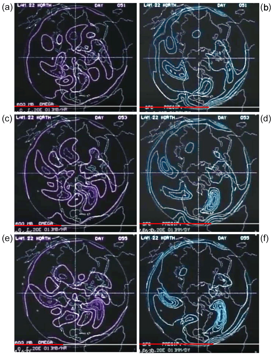
Figure 3 Snapshots from the computer animation showing LAM results at three times near 12Z on days 51 (a, b), 53 (c, d), and 55 (e, f). Panels (a), (c), and (e) show the pressure vertical velocity (dashed contours denote negative values, i.e., upward motion), and panels (b), (d), and (f) show the precipitation rate.

The animation includes a point moving westward around the outside of the polar projection each day that presumably marks the longitude of the subsolar point. The daily variations of 500 hPa heights and surface pressure are easily seen in the tropics – notably, it is apparent that the changes in these fields are dominated by a semidiurnal component. This variation is discussed in the next section.

7 LAM simulation of atmospheric tides

One aspect of the LAM that notably attracted attention was the diurnal cycle in the tropics whose features could be seen directly in Leith's animations. The interest of Hunt and Manabe (1968) in the atmospheric tide apparent in the LAM animation has been noted earlier. In his interview with Edwards (1997), Leith notes the interest in the atmospheric tide in LAM from those viewing his animations:

But the other things that showed up that are interesting on the film, like 12-hour tide of especially cloud cover, which is still something … people have talked a lot about atmospheric tides, but nobody knew very much about what they were. There is some evidence of the amplitude of these tides, but this actually right away showed one. It was kind of interesting in that regard. But mostly, well, mostly it just got people to see… This is the 500 millibar height field … there you can see rather clearly the tide. It's a 12-hour tide in fact … it's in the tropics that the tide shows up the most.

In Hundebol (2013), MacCracken is quoted as saying the following:

Leith did some experiments with the atmospheric model. One of the things he did in the model, of course, was he had day and night! GFDL didn't do that for another, I don't know, 12 years or something like that… He had day and night, and the model showed a semidiurnal tide [in equatorial latitudes], which is something that is observed… So that was kind of a fascinating result from a model in the early 1960s.

It is also noteworthy that the only published quantitative analysis of any of the LAM output is apparently the study of the atmospheric tides in Hardy (1968).

A simple plot of hourly barometric observations from any low-latitude location in the real world will show a very prominent solar semidiurnal (12 h) tidal harmonic with a surface pressure amplitude at the Equator of ∼1.2 hPa and a rather coherent sun-synchronous propagation (so that maximum pressure is typically observed around 10:00 and 22:00 LT, local time). This was, of course, well known even in the 19th century, but in the early 1960s the prominence of the 12 h tide was still a major unsolved mystery (Chapman and Lindzen, 1970). At low latitudes, the 12 h pressure tide is at least twice as large as the 24 h tide despite the solar heating projecting much more strongly onto the 24 h harmonic (∼5 times as much heating as in the 12 h harmonic). In the late 19th century, Lord Kelvin noted that the prominence of the 12 h tide could be explained if the atmosphere had a natural resonant period near 12 h, and this resonance hypothesis held sway until the late 1940s when the first in situ observations of mesospheric temperatures revealed that the atmosphere did not have a free oscillation of a 12 h period (Chapman and Lindzen, 1970). Therefore, at the time when the LAM was developed in 1960, the prominent 12 h tide remained a long-standing mystery. Thus, it is understandable that scientists at the time were impressed when it was shown that the LAM spontaneously simulated a fairly realistic atmospheric tidal signal at the surface.

Hardy (1968) reported on his analysis of 3-hourly surface pressure data from 16 consecutive days of an integration of a Northern Hemisphere version of LAM. He found that the 12 h harmonic had an amplitude of about 0.9 hPa at the Equator and peaked around 10:15 LT (and 22:15 LT), while the 24 h harmonic had an amplitude of ∼0.25 hPa and peaked around 04:00 LT. In the mid-1960s there had been some key developments in the theory of the atmospheric tide (see Chapman and Lindzen, 1970), and by 1968 it was known that an important forcing for the semidiurnal tide was the direct absorption of solar radiation by ozone in the stratosphere. This led Hardy himself to wonder how the LAM, with its lack of radiative heating above the 50 hPa top level, was able to come close to a realistic amplitude:

The LAM code is somewhat deficient in that no upper atmospheric physics are included. Since upper atmospheric effects are known to affect the tides, the LAM results are to be interpreted only as representing the component of the tides due to the part of the atmosphere below 68,000 feet.

Much later, a more complete study of the solar atmospheric tide in an AGCM was conducted by Zwiers and Hamilton (1986) who noted that the typical upper boundary condition in AGCMs prevents the propagation of tidal energy into the upper atmosphere, resulting in an artificial enhancement of the tide in the lower atmosphere and at the surface. It is plausible that this artificial enhancement of the tide in LAM largely compensated for the lack of the upper stratospheric solar heating tidal excitation.

8 Conclusion

The development of the LAM virtually single-handedly by Leith was a very impressive accomplishment and a very notable step forward in creating tools for environmental prediction. As shown here, it is reasonable to suppose that the LAM was running by late 1960; thus, it has a claim to be the first (by some years) comprehensive atmospheric simulation model with (i) multiple levels in a domain spanning the troposphere and even the lowermost stratosphere, and (ii) a representation of the hydrological cycle and clouds. It is consequently reasonable to regard the LAM as the first numerical model that can claim to be an AGCM.

Despite an early start, Leith's work in developing the LAM proved much less influential in the long run than the projects to develop climate simulation models at GFDL, UCLA, and NCAR, and the LAM effort left almost no direct footprint in the scientific literature. However, Leith's work was inspirational to the other pioneering groups at a critical time for climate model development (it also left a legacy as the starting point for developing a two-dimensional atmospheric circulation model that was applied in climate studies as late as the 1980s). Leith's techniques for producing animated movies displaying his model results were copied by his competitors, and Leith's contributions stand at the very beginning of the ever-evolving field of computer visualization of atmospheric circulation.