the Creative Commons Attribution 4.0 License.
the Creative Commons Attribution 4.0 License.
 | 20 Mar 2020
Tide prediction machines at the Liverpool Tidal Institute
The 100th anniversary of the Liverpool Tidal Institute (LTI) was celebrated during 2019. One aspect of tidal science for which the LTI acquired a worldwide reputation was the development and use of tide prediction machines (TPMs). The TPM was invented in the late 19th century, but most of them were made in the first half of the 20th century, up until the time that the advent of digital computers consigned them to museums. This paper describes the basic principles of a TPM, reviews how many were constructed around the world and discusses the method devised by Arthur Doodson at the LTI for the determination of harmonic tidal constants from tide gauge data. These constants were required in order to set up the TPMs for predicting the heights and times of the tides. Although only 3 of the 30-odd TPMs constructed were employed in operational tidal prediction at the LTI, Doodson was responsible for the design and oversight of the manufacture of several others. The paper demonstrates how the UK, and the LTI and Doodson in particular, played a central role in this area of tidal science.
- Article
(4770 KB) - Full-text XML
- BibTeX
- EndNote


In the year following the end of the First World War, a number of organisations were established which have had a lasting importance for geophysical research. At an international level, the International Union of Geodesy and Geophysics (IUGG) was founded in that year (Joselyn and Ismail-Zadeh, 2019). The 100th anniversary of the IUGG, which remains the pre-eminent international body for geophysics, has been marked by a series of papers in a special issue of this journal (entitled “The International Union of Geodesy and Geophysics: from different spheres to a common globe”).
An example of an important development for geophysics at a national level was the establishment of the Liverpool Tidal Institute (LTI), marked by the set of papers in another special issue of this journal (entitled “Developments in the science and history of tides”). The LTI was based initially at Liverpool University with Joseph Proudman as honorary director and Arthur Doodson as secretary. However, by 1929 it had relocated across the river Mersey to Bidston Observatory where there was more room for research and where Doodson took up residence as associate director (Nature, 1928). It was renamed the Liverpool Observatory and Tidal Institute, and during the next 100 years there were to be several other changes of name including the Proudman Oceanographic Laboratory. The LTI (as I shall continue to call it for the purpose of this paper) became an acknowledged centre of expertise for research into ocean and earth tides, storm surges, sea level changes (Permanent Service for Mean Sea Level), and the measurement and modelling of coastal processes.
Some of the history behind the establishment of the LTI is described by Carlsson-Hyslop (2010, 2020). Short histories may also be found in Doodson (1924) and Cartwright (1980, 1999). The present paper focuses on one area of work for which the LTI became renowned, the development of tide prediction machines (TPMs). Arthur Doodson (1890–1968) was the main person involved in this aspect of the LTI's history, and so he is the main character of interest for the present paper (Fig. 1a). Scoffield (2006) and Carlsson-Hyslop (2015) contain details of his early career. Proudman (1968) provides an excellent overview of many aspects of Doodson's research at the LTI, including that with the TPMs (see also Cartwright, 1999).
TPMs were analogue computers which, before the advent of digital computers, provided an accurate and efficient means of predicting the ocean tide, and in particular they predicted the heights and times of high and low waters reported in tide tables. Cartwright (1999) gives a general explanation of TPMs and provides a description of some of them, while Hughes (2005) contains some of the history of the individuals associated with them.
The first TPM (aside from prototype models) was designed by Sir William Thomson (1824–1907, Baron Kelvin of Largs from 1892; Fig. 1b), with the help of Edward Roberts from the UK Nautical Almanac Office, and was constructed by the scientific equipment company of Alexander Légé in 1872–1873 with funding from the British Association for the Advancement of Science (BAAS). Therefore, all TPMs are sometimes referred to as “Kelvin machines”, although this name is also used to refer to a particular type of TPM (see below). Between the 1870s and 1960s, over 30 TPMs were constructed around the world, of which the majority were made in the UK. Only three of them were used for tidal prediction at the LTI. However, there were more for which Doodson played a major role in their design. In addition, he supervised closely their manufacture by the Légé company and provided a certificate of efficiency prior to delivery to customers. As a consequence, the LTI played the central role between the 1920s and 1960s in this area of tidal science.
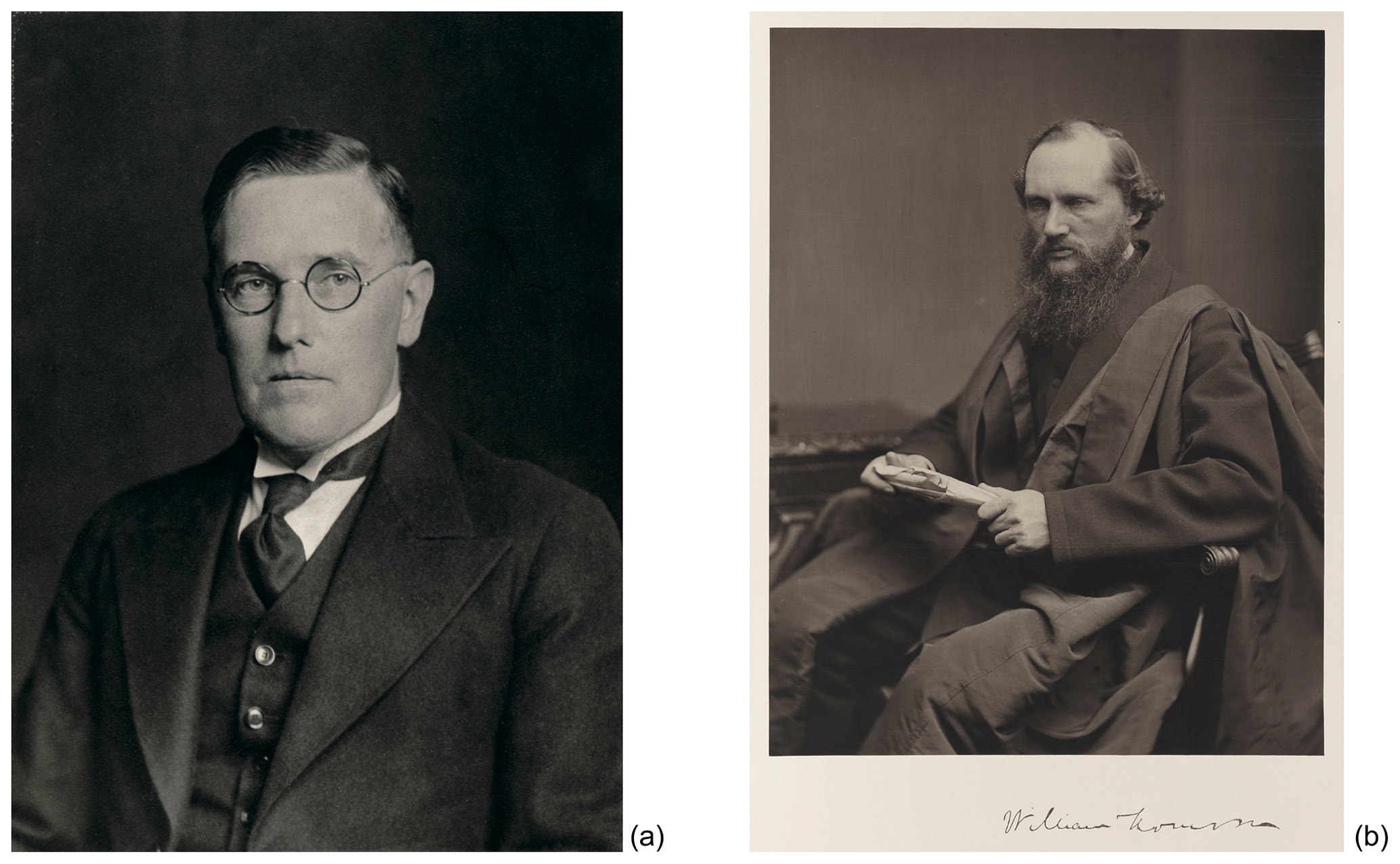
Figure 1(a) Arthur Thomas Doodson CBE, DSc, FRS, FRSE (1890–1968) photographed in 1933 by Walter Stoneman. (b) Sir William Thomson (1st Baron Kelvin of Largs) OM, GCVO, PC, FRS, FRSE (1824–1907) photographed in 1871 by Thomas Annan. © National Portrait Gallery, London.
Cartwright (1999) contains a comprehensive description of the history of tidal science from antiquity to the present day. During most of the 19th century, tide tables in the UK were produced using the non-harmonic or “synthetic” method developed by Sir John Lubbock (Baron Avebury) (Rossiter, 1971; Durand-Richard, 2016a). That method worked well in areas with predominantly semidiurnal tides, and in fact the Admiralty continued to use non-harmonic methods derived from Lubbock's work well into the 20th century (Rossiter, 1971). However, it was less suitable in regions with proportionately larger diurnal tides such as along the coastlines of India and Australia. Another disadvantage of Lubbock's method was that it required the use of long tide gauge records, such as those from London or Liverpool (e.g. Lubbock, 1835). These deficiencies led to the development of the harmonic method in the 1860s, first by Kelvin aided by Roberts, and then also by Sir George Darwin (the second son of Charles Darwin) and others, under the auspices of the BAAS. The harmonic method's advantage of being able to use short tide gauge records (i.e. a year or less) ultimately enabled tidal predictions to be produced for ports located in any tidal regime.
Using the harmonic method, the tide at any one location can be described with good accuracy as an expansion in terms of a number (N) of “constituents” or “satellites” such that
where the total tide htotal at time t is expressed as a sum of one cosine for each constituent; ωi is the angular speed of constituent i; , where Ti is its period; and hi and gi are its amplitude and phase lag. N is infinite in principle but, in practice, the ocean tide can be described with good accuracy at most open-ocean locations by several 10 s of constituents.1
Consequently, if one has prior knowledge of each ωi, hi and gi, then one can calculate the height of the tide at any time t from the set of cosines. How one acquires this prior knowledge will be explained below. The “turning points” of the tidal curve (when ) will provide the heights and times of high and low waters.
One could undertake such a tedious arithmetic computation oneself, by calculating the height of the tide every hour during the year, by plotting the resulting time series and by inspecting the plot to see when the turning points occur and what their heights are. However, it was Kelvin's realisation that TPMs could provide a means for undertaking such a task more efficiently, their accuracy being limited only by the number of constituents or “components” (N) included in their design, that led to their development and use in tidal prediction up until the 1960s.2 Kelvin's first machine (the so-called “British Association Machine”), derived from a device used in telegraphy by Sir Charles Wheatstone, could simulate a tide containing 10 constituents. Later machines included many more, as shown in Table 1a. The largest accounted for 62 harmonic constituents. That is the enormous machine, weighing 7 t, designed in Germany by Heinrich Rauschelbach and now on display at the Deutsches Museum in Munich (Cartwright, 1999). It is denoted as TPM-S16 in Table 1a. Although open-ocean tides could be predicted effectively in this way, Doodson was always rightly sceptical about the ability of TPMs to simulate tides in estuaries, even when N was large (Doodson, 1926).
Table 1(a) Inventory of tide prediction machines. (b) Inventory of portable tide prediction machines.
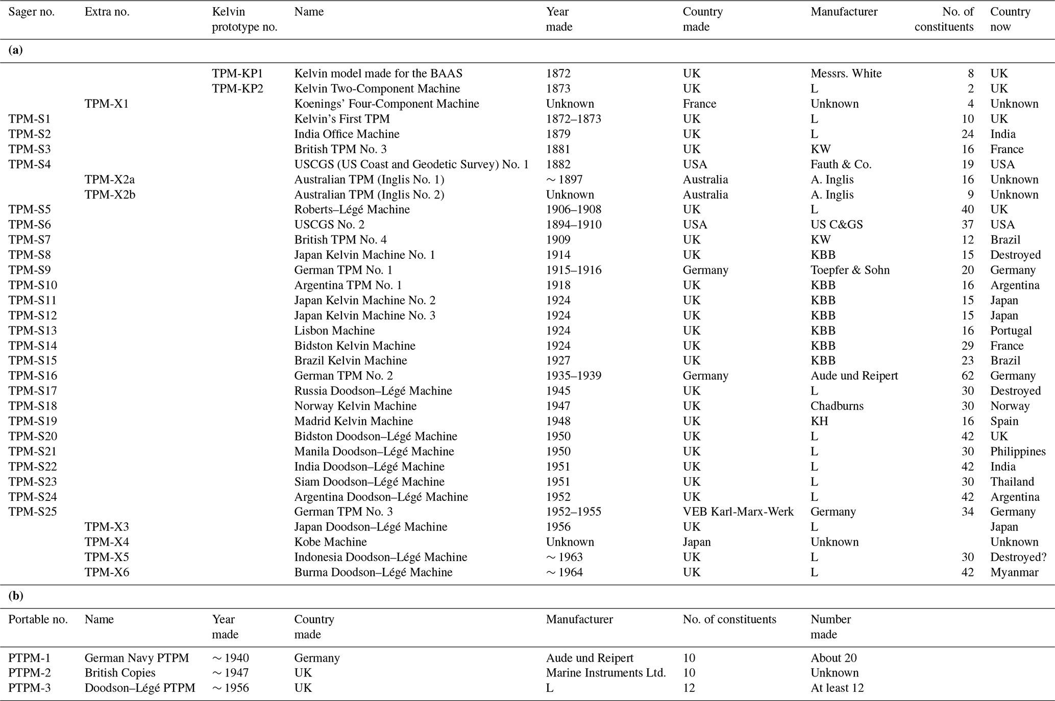
Manufacturers: L – Alexander Légé & Co.; KW – Kelvin and White, Glasgow; KBB – Kelvin, Bottomley and Baird, Glasgow; KH – Kelvin and Hughes, Glasgow.
Each TPM had its own architecture (as a modern computer scientist might say). However, there were several features common to almost all of them. First, one had to have a driving mechanism (either by hand or electric motor) to provide a circular motion with an angular frequency ωi corresponding to that of a tidal constituent. Second, one required a mechanism for converting that circular motion into sinusoidal motion. Third, one had to sum the individual sinusoidal motions to derive an overall sum as in Eq. (1).
The important angular frequencies (ωi) associated with the tide have been known for many years from astronomical measurements of the motions of the sun and moon (e.g. see chap. 8 of Cartwright, 1999). A TPM mechanism includes crank wheels which revolve at frequencies for each individual constituent relatable to the actual frequencies of the constituents of the tide in the ocean via a scaling factor designed into the machine. In practice, this is impossible to do precisely, but the integer number of teeth on the various wheels can always be selected such that a constituent's frequency in the machine is as close as possible to that required in the ocean tide (times the scaling factor). This sort of choice of number of teeth for any required gear ratio within a machine such as a TPM is a well-understood engineering problem; this task was addressed by Roberts for Kelvin during the design of the first TPM. However, the inherent imprecision limits the ability to use TPMs to make predictions over many years, as do mechanical issues such as friction within the mechanism (Doodson, 1926; Doodson and Warburg, 1941). Instead, the machines usually have to be set up again for every year of prediction; see below. Similarly, the amplitude within the mechanism associated with a given constituent has to be relatable to its known value hi multiplied by another scale factor defined by the way the machine is set up. In addition, the phase of sinusoidal motion of each constituent in the machine has to be consistent with the phase lag of that constituent in the real ocean tide. Many practical aspects involved in the construction of a working TPM are described in chap. 14 of Doodson and Warburg (1941).
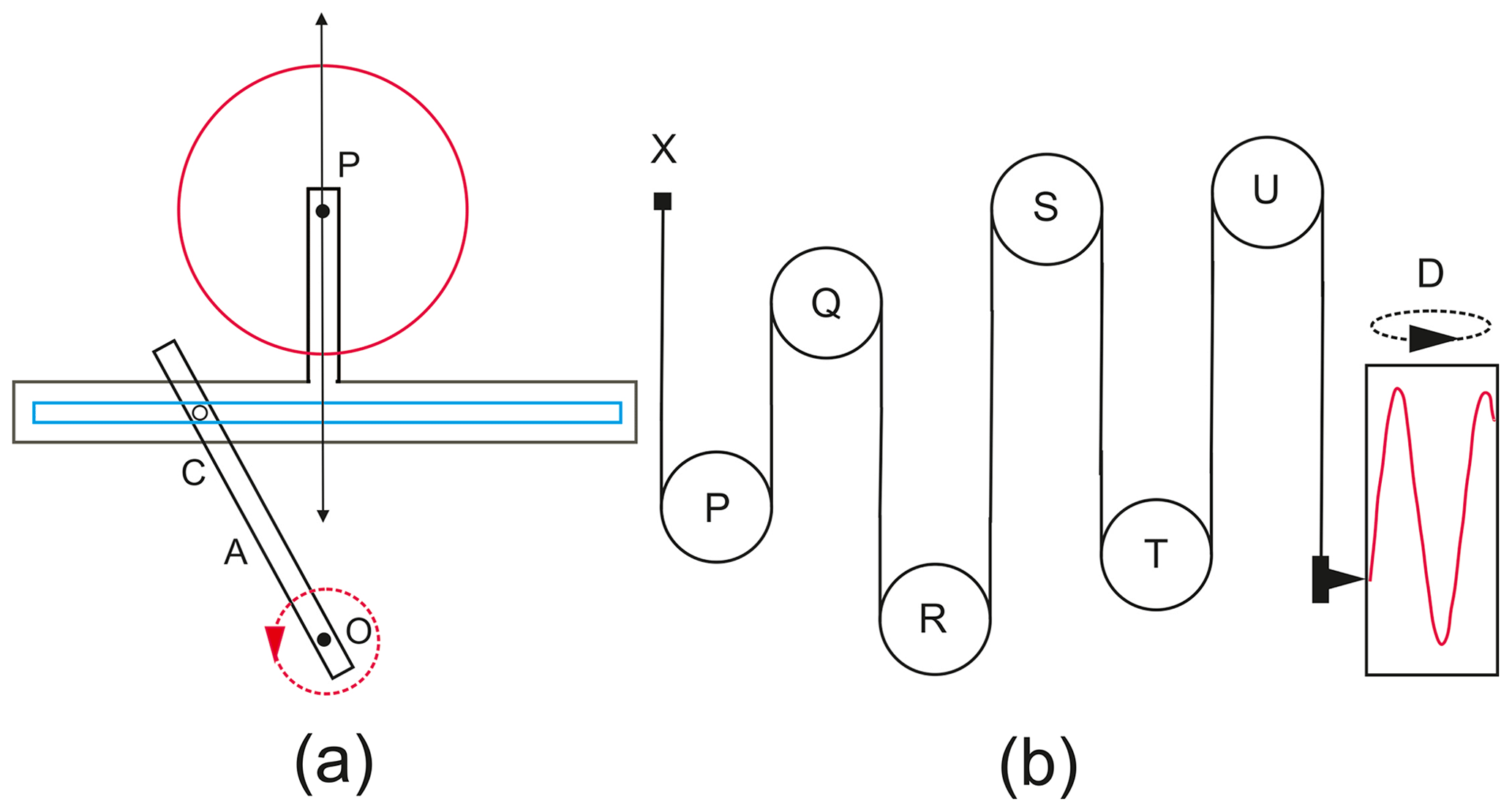
Figure 2Schematic figure of a TPM based on drawings in Doodson and Warburg (1941). (a) A method for producing vertical sinusoidal motion corresponding to that of one tidal constituent and (b) a method for summing six constituents with the use of a band wrapping around each pulley. See the text for further explanation.
Figure 2 is adapted from drawings in Doodson and Warburg (1941) (see also a similar drawing in Cartwright, 1999). It provides a schematic example of how most of the TPMs worked, with the various components described above. Figure 2a indicates the circular motion of a crank A revolving around a centre O, with a pin C fixed in the crank, which is free to move along a horizontal slot in a T piece. The T piece itself is allowed to move up and down in a vertical direction only. Therefore, its elevation will vary by OC cos (COP). (The width of the slot obviously has to be larger than twice OC). It can be appreciated that OC can be related to the amplitude of a constituent, with the rate of revolution of the crank proportional to the constituent's angular speed and that an initial angle at t=0 must be capable of being set to represent the phase lag. Then, as the crank rotates, a pulley wheel centred at P connected to the T piece will rise and fall, thereby simulating the variation in water level due to that constituent. A number N of such units (six in the case of Fig. 2b) can be geared to a main shaft so that the individual speeds are proportional to those of the six constituents. This is achieved by means of the number of teeth in the gear wheels. All motions are summed by using a continuous tape (or “band”) usually made of a metal such as nickel. The band is fixed at one end X and wraps around the six pulleys P–U. At its other end it has a pen carriage which plots a trace on a paper chart on a rotating cylinder D. Section 7 describes how a real machine, in this case the Bidston Doodson–Légé Machine (TPM-S20 in Table 1a; Doodson, 1951, 1957), can be set up for each year of prediction required. This is done by adjusting wheels located on the face of the machine for the known amplitudes and phases of each constituent, similar to those shown schematically in Fig. 2b.
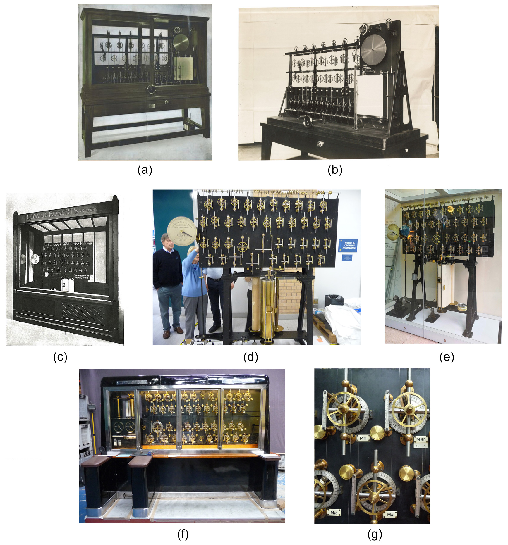
Figure 3Photographs of the three Bidston TPMs: (a) the Bidston Kelvin Machine as normally seen in its casing and (b) an earlier photograph showing more clearly the machine components, including the wheels for each tidal constituent and, on its right-hand side, the chart plotter. (Photos: National Oceanography Centre and SHOM.) (c) The Roberts–Légé Machine at the Franco–British Exhibition of 1908, (d) being refurbished in 2015 and (e) on display at NOC in Liverpool in 2019. (Photos: National Oceanography Centre, Philip Woodworth and Helen Rawsthorne.) And (f) the Bidston Doodson–Légé Machine after being refurbished in 2015 with (g) a close-up of the pulley wheels for the M10, Mm, M8 and MSf constituents between which a nickel band can be seen passing over or under each pulley. Each amplitude block contains a Vernier screw with which to set the constituent's amplitude, while its phase is defined using the wheel behind. The brass knobs are the clutch controls for each constituent. (Photos: Philip Woodworth.)
The most obvious product of the TPM was the ink trace on a paper chart, similar to that produced by a traditional float and stilling well tide gauge equipped with a chart recorder. The fluctuations in the tide-like trace on the chart were proportional to those in the real ocean with a constant of proportionality set by the machine design.
However, in practice, what most people needed to know was simply the heights and times of high and low waters, not a continuous time series given by a trace on a chart. The procedure for providing this information using most machines was to set up the machine for use in two stages. In a first stage, the individual sinusoidal motions would be arranged not as cosines summing to htotal but as a sum of the individual rates of change of height.
The machine operator would run the machine, set up for the year required for prediction, and note the times t when happened to be zero, usually four times per day. The machine would then be set up so as to provide Eq. (1), and the operator would make a note of the heights corresponding to each turning point time t. The operator would then have all the information required for a tide table.
If funds allowed, then it was highly desirable to have a TPM that was double sided. In this case, the machine was two machines in one, with one side calculating the rates and the other side the heights (Eqs. 2 and 1 respectively). Instead of a paper chart, the instantaneous rates and heights at time t would be displayed on a panel on the front of the machine, and the operator would simply have to note the heights and times when rates were zero. As a result, there was a major improvement in the overall efficiency of the work. The Bidston Doodson–Légé Machine (TPM-S20) provides a good example of this. When first constructed in 1950 it was a single-sided machine, until funds could be made available in 1956 to enable its conversion to a double-sided machine.3
Figure 2 provides only a schematic description of a TPM. However, while the principles of construction of each machine were much the same, their mechanical design differed in detail. Therefore, if one looks into aspects of a particular machine now, it may be difficult to obtain a complete understanding without access to copious original documentation.
An updated “inventory” has been made recently of all the TPMs that were made by various groups around the world (Woodworth, 2016). Tables 1 and 2 are based on the corresponding tables in that report.
A first inventory was made by the International Hydrographic Bureau in 1926 (IHB, 1926).4 This was a collection of sets of information provided by the machine owners at the time. However, Arthur Doodson remarked that the report could have been done better (Doodson, 1926). A second inventory was made in 1955 by the oceanographer Günther Sager from Germany. Chapter 3 of his “Gezeitenvoraussagen und Gezeitenrechenmaschinen” is entitled “Zur geschichtlichen Entwicklung der Gezeitenrechenmaschinen” or “The Historical Development of Tide Calculators”. It contains a list of the 25 TPMs that he knew about and gives some technical details of each one. In this case, it is known that Sager corresponded with Doodson and received help in the compilation of his inventory.
Table 1a contains a line for each TPM with a code number such as TPM-S20, indicating that the machine was number 20 in Table 2 of Sager (1955); TPM-KP1, indicating Kelvin's first prototype; TPM-X1, indicating a machine that was not in Sager's 1955 inventory; or PTPM-1, indicating the first portable tide prediction machine (PTPM). Sager did not include the prototype machines of Kelvin, presumably because they were never used for operational tidal predictions. In addition, there were a couple of omissions such as the two Australian TPMs. His book was published in 1955, just as the production of the machines was coming to an end, but there were still at least three to come along, including the Japan, Indonesia and Burma (Myanmar) Doodson–Légé machines denoted TPM-X3, X5 and X6 in Table 1a. In addition, he did not include the smaller portable TPMs that were developed for military and hydrographic surveying purposes; those that I know about are listed in Table 1b. As far as I know, they were not a great success and never became as well-known as the larger machines.
Table 2Lord Kelvin Tide Predictors. The machines made by the Kelvin companies carried plaques that gave the machine a “Lord Kelvin Tide Predictor” number. This table provides a list of these machines.

Table 1a includes each machine name and the year and country of its manufacture, together with the manufacturer's name. It also shows the number of constituents in its design and the country where the machine is now located. Woodworth (2016) contains more details for some of them. For example, when a machine was refurbished, extra constituents were sometimes added, such as the conversion from 20 to 24 constituents for TPM-S2 during its refurbishment in 1891.
It can be seen from Table 1a that most of the machines were associated with a particular manufacturer and so with a particular architecture. As mentioned above, the invention of the TPM is usually credited to Kelvin and all TPMs are sometimes called Kelvin machines. However, “Kelvin-type” machines can also refer simply to the set of machines made in Glasgow (also in London and Basingstoke) by companies that were associated with Kelvin or, after his death, continued to carry his name (Table 1a). These “Lord Kelvin Tide Predictors” are referred to further in Table 2. The Norway Kelvin Machine (TPM-S18) was also a Kelvin type, although it was made by Chadburns of Liverpool and not by one of the Kelvin companies.
In addition, there were a number of machines, following the Roberts–Légé Machine of 1906 (TPM-S5), that could be described as “Légé type” (or “Roberts–Légé type” or “Doodson–Légé type”). This applies to the later machines, designed or supervised by Edward Roberts or Arthur Doodson. These were manufactured by the London scientific equipment company of Légé & Co. The Kelvin and Légé type architectures were quite different, the companies retaining those distinctive architectures for many years. For example, the Roberts–Légé Machine (TPM-S5) and the Doodson–Légé Machine (TPM-S20), made a half-century apart by the Légé company, have a similar number of constituents and look very similar. However, the Légé-type machines tended to be more solid in construction, with moving parts for the harmonic motion made in steel instead of brass, and therefore they were more expensive.
Although there were important TPMs constructed in Germany and the USA (USCGS, 1915; Hicks, 1967; Cartwright, 1999; NOAA, 2019), the majority were designed and manufactured in the UK. Of the 33 machines in Table 1a, 25 of them were made in either London, Glasgow or Liverpool. In addition, the UK was the only country to export TPMs to other countries. The construction of the majority of the machines made after 1920 was supervised, one way or other, by Arthur Doodson. He oversaw the construction by Légé of machines for Russia, Bidston, Philippines, India, Thailand, Argentina and Japan (TPM-S17, S20–S24 and X3) and provided advice to prospective purchasers of other machines, such as that made for Norway by Chadburns (TPM-S18).5 Those that he inspected were awarded a “Certificate of Efficiency”. The Russia Doodson–Légé Machine (TPM-S17) required a particular effort, involving many trips by Doodson from Bidston to the Légé factory in London during wartime. Such travel was essential, as Légé had not made a similar machine for almost half a century since TPM-S5. It is unfortunate that the Russia Doodson–Légé Machine is one of the few machines not to survive, although in fact it is the only one for which there is a historical record on film (Tide and Time, 2019). The so-called Siam (Thailand) Doodson–Légé Machine (TPM-S23) was made to a particularly high standard and was displayed in the “Dome of Discovery” at the Festival of Britain in 1951.
After Doodson's retirement in 1960, the liaison with Légé was taken over by Jack Rossiter, the new director at Bidston. This included the manufacture of machines for Indonesia and Burma (TPM-X5 and X6). Scoffield (2006) mentions that Légé & Co. may have also been trying to sell another machine to Mexico in early 1965 and was unhappy when Rossiter suggested selling them the Roberts–Légé Machine (TPM-S5) instead. However, neither proposal came to anything, and subsequently Bidston terminated its relationship with Légé on the advice of the solicitors of Liverpool University owing to the company's financial difficulties.
TPMs provide just one example of how analogue machines undertook routine mathematical tasks in a wide range of scientific research before digital computers became available, and Tables 1 and 2 show that they were employed by tidal agencies in many countries. Rawsthorne (2019) has conducted a “prosopographical study” of this entire inventory of TPMs, in a study of how ideas and technology are spread around the world. Analogue machines continue to have an important role in many modern research fields (MacLennan, 2018).
Most of the funding for the establishment of the LTI in 1919 had come from Sir Alfred Booth and his brother Charles Booth of the Booth Shipping Line in order to “prosecute continuously scientific research into all aspects of knowledge of the tides” (Doodson, 1924; Carlsson-Hyslop, 2020).
In 1925, Charles Booth also provided most of the GBP 1500 required for the purchase of a 25- to 28-component TPM for the exclusive use of Doodson at the LTI. The BAAS contributed GBP 300. In the event, this became a 26-component machine, later extended to 29 components. This Bidston Kelvin Machine (TPM-S14) was made by the firm of Kelvin, Bottomley and Baird of Glasgow with Doodson taking a great interest in its construction and suggesting modifications. It stood about 7 feet (2.1 m) high, 6 feet (2 m) long and 2 feet (0.6 m) wide and was encased by sliding doors (Doodson, 1925, 1926, 1927). Figure 3a and b show photographs of the machine.
Then in 1929, following the death of H. W. T. Roberts (the son of Edward Roberts), Doodson acquired the Légé-made machine that Edward Roberts had designed in 1906 and which had won a Grand Prix at the Franco–British Exhibition of 1908. Roberts had subsequently used it as part of his own tidal prediction business (Messrs. Edward Roberts & Sons of Broadstairs), with the work of that business, including predictions for the Hydrographic Office, also passing to the LTI in 1929. Doodson paid the Roberts family GBP 753 15s 0d. This Roberts–Légé Machine (TPM-S5) simulated 33 constituents, several more than the Bidston Kelvin Machine. By 1929 it was in need of an overhaul and refurbishment. Shortly thereafter, the number of constituents was increased to 40 by Chadburns of Liverpool, with its original design having allowed for such a future expansion. Its dimensions are approximately 7 feet (2.1 m) high, 6 feet (2 m) long and 2.5 feet (0.8 m) wide (somewhat wider with its casing). It remained in use at Bidston until 1960 (Scoffield, 2006). This TPM was sometimes known as the “Universal Tide Predictor of 1906” and also as the “Roberts Tide Predicting Machine”, a name which had previously been attached to the India Office Machine (TPM-S2) which had also been designed by Roberts. Doodson and Bidston staff referred to it as the “Légé machine”. Photographs of this machine are shown in Fig. 3c–e.
Doodson wrote in an internal note that there was no difference in performance between the Bidston Kelvin and Roberts–Légé machines. He stated that for both “the total error of production of a tide does not differ by more than 0.05 ft (1.5 cm) and 1 min of time from calculations using the same harmonic constants, even for the largest ranges of tide”.
These two TPMs equipped Doodson with experience that would prove invaluable when considering the design of later machines. They would also provide him with the means to enable the LTI to become one of the main producers of tide tables worldwide. The two machines were to play particularly important roles in World War II, in providing tidal predictions for D-Day and for other military operations in Europe and the Pacific. Those for D-Day were unusual in that they were made for an unknown location (now of course known to be Normandy), using only the crudest of harmonic constants provided by Commander Farquharson at the Tidal Branch of the Admiralty (Parker, 2011). However, they were not secret for long. In July 1944, Doodson gave a lengthy interview to the Liverpool Daily Post, stressing the importance of the TPMs to the D-Day predictions (LDP, 1944).
In 1947, Doodson asked Légé to estimate the price of a machine with at least 35 components. Légé produced an initial design which Doodson started working on in detail. This became the 42-component machine delivered finally by Légé in December 1950 at a cost of GBP 5049 (Woodworth, 2016).6 This Bidston Doodson–Légé Machine (TPM-S20), referred to by Bidston staff as the “D–L machine”, was the third machine to be used operationally at the LTI and one of a number of similar machines made by Légé & Co. under Doodson's supervision and exported to several countries. Doodson (1951) describes it in some detail. It was a single-sided TPM, being converted to a double-sided machine in 1956. It has an aluminium frame, unlike the steel frame of TPM-S5. The machine is approximately 7 feet (2.1 m) high, 9.5 feet (3 m) long and 3.5 feet (1.1 m) wide and weighs 1.4 t (not including the support base frame). Complete engineering drawings and documentation survive which have enabled its recent restoration.7 Figure 3f and g provides photographs of the machine.
The purchase of the Doodson–Légé Machine had been made contingent on the sale of the Bidston Kelvin Machine to the Service Hydrographique et Océanographique de la Marine (SHOM) in France. It was acquired by them in 1950 and was operated first in Paris and then in Brest for predicting the tides of overseas ports (SHOM, 2019). It remained in operational use at SHOM until 1966 (Rawsthorne, 2019). Nowadays, the Roberts–Légé and Doodson–Légé machines are both on display at the National Oceanography Centre in Liverpool (Tide and Time, 2019), the only place in the world where two TPMs can be seen alongside each other. Meanwhile, the Bidston Kelvin Machine may still be found at SHOM in Brest. All three machines are in working or near-working order.
Equation (1) shows that if one knows the amplitudes and phases of each constituent at a point on the coast (known collectively as the “harmonic constants” for that location), then it is possible to compute the total tide htotal at that position for any time t, either by considerable arithmetic effort or with the use of a TPM. However, how does one know the harmonic constants in the first place?
Any calculation of the harmonic constants has to be based on measurements made at the location by a tide gauge, providing a record of the sea level at every hour (for example) for an extended period such as a month or year. At one time, there were hopes that machines could perform a harmonic analysis of each record, machines having been invented during the 19th century to undertake many mathematical tasks (De Mol and Durand-Richard, 2016). Kelvin applied the Disk-Globe-and-Cylinder Integrator developed by his brother, James Thomson, to the evaluation of the integrals needed for harmonic analysis and thereby to the determination of harmonic constants from an input time series of tidal measurements. Kelvin called this “substituting brass for brain” (Thomson, 1881).
A small number of such machines were made eventually. Kelvin first constructed a model of a five-component machine capable of analysing a time series from which one could determine the cosine and sine components of two harmonic constituents together with a mean value. This machine is now on display at the Hunterian Museum of Glasgow University. A similar machine made by R. W. Munro and Company was employed by the Meteorological Office for the determination of daily variations in meteorological parameters (Thomson, 1878); this is now on display at the Science Museum. However, for tides one needed a machine capable of handling more harmonic terms. By 1879, an 11-component machine had been made, specifically for application to tides (Thomson and Tait, 1879; Thomson, 1881). It was not a great success. Thomson and Tait (1879) remarked that “The machine has been deposited in the South Kensington Museum”. Parts of it are now preserved in the Science Museum store; a photograph of it is contained in De Mol and Durand-Richard (2016). 8 Proudman (1920) and Hughes (2005) mention several later attempts at mechanical tidal analysers, although they do not seem to have been successful either. Of course, by then the numerical methods of tidal analysis devised by Darwin (1893), and later developed by Doodson (1928) discussed below, had removed the necessity for mechanical analysers. However, the use of similar machines for mechanical harmonic analysis has continued to attract interest in science and engineering through the years (e.g. Webb and Bacon, 1962, and for a review see Durand-Richard, 2016b, Sect. 8.2.3).
The harmonic analyser was a classic example of Kelvin's ingenuity. However, the machine had no lasting importance within tidal science, and, in the context of the present paper, it was not relevant to the work of the LTI. Instead, the harmonic constants had to be determined by laborious arithmetical methods by teams of (predominantly female at the LTI) assistants called “computers” (Fig. 4). In the following, I outline the method developed at the LTI by Arthur Doodson and put into practice by his team of computers. 9
Before doing that, it is useful to recall that the two largest tidal constituents in many parts of the world are M2 (the main semi-diurnal tide from the moon with a period of 12 h 25 min, half a lunar day) and S2 (the main semi-diurnal tide from the sun with a period of 12 h, half a solar day). Most other constituents also have periods around either 12 or 24 (semi-diurnal and diurnal tides), while some have shorter periods (shallow-water tides), and a few have periods of up to a year or more (long-period tides). Ideally, all of the most important of these constituents need to be represented in the mechanism of a TPM, requiring prior knowledge of the harmonic constants.

Figure 4A group photograph of the team of computers at Bidston Observatory in 1953. (Photo: Valerie Gane.) They are gathered around the original Liverpool One O'Clock Gun which, when located in Birkenhead Docks, was fired by means of transmission of an electrical signal from the Observatory.
For present purposes, I focus on the derivation of the semidiurnal constants and use Liverpool as an example. At this location, M2 and S2 have amplitudes of 3.13 and 1.01 m respectively. Because a solar day lasts 24 h, the S2 tide will repeat itself twice a day exactly at the same time every day (shown in red in Fig. 5a). M2 has a larger amplitude and repeats twice a lunar day (a little later each solar day), as shown in blue. They combine by “beating together”, resulting in a total tide that is larger and smaller over a fortnight (spring and neap variation, Fig. 5b). The separate contributions of M2 and S2 to the total tide would not be readily apparent with just 1 d of data, but the fact that they both exist becomes obvious when looking at this simple variation over a fortnight. However, the existence of other semidiurnal constituents complicates things.
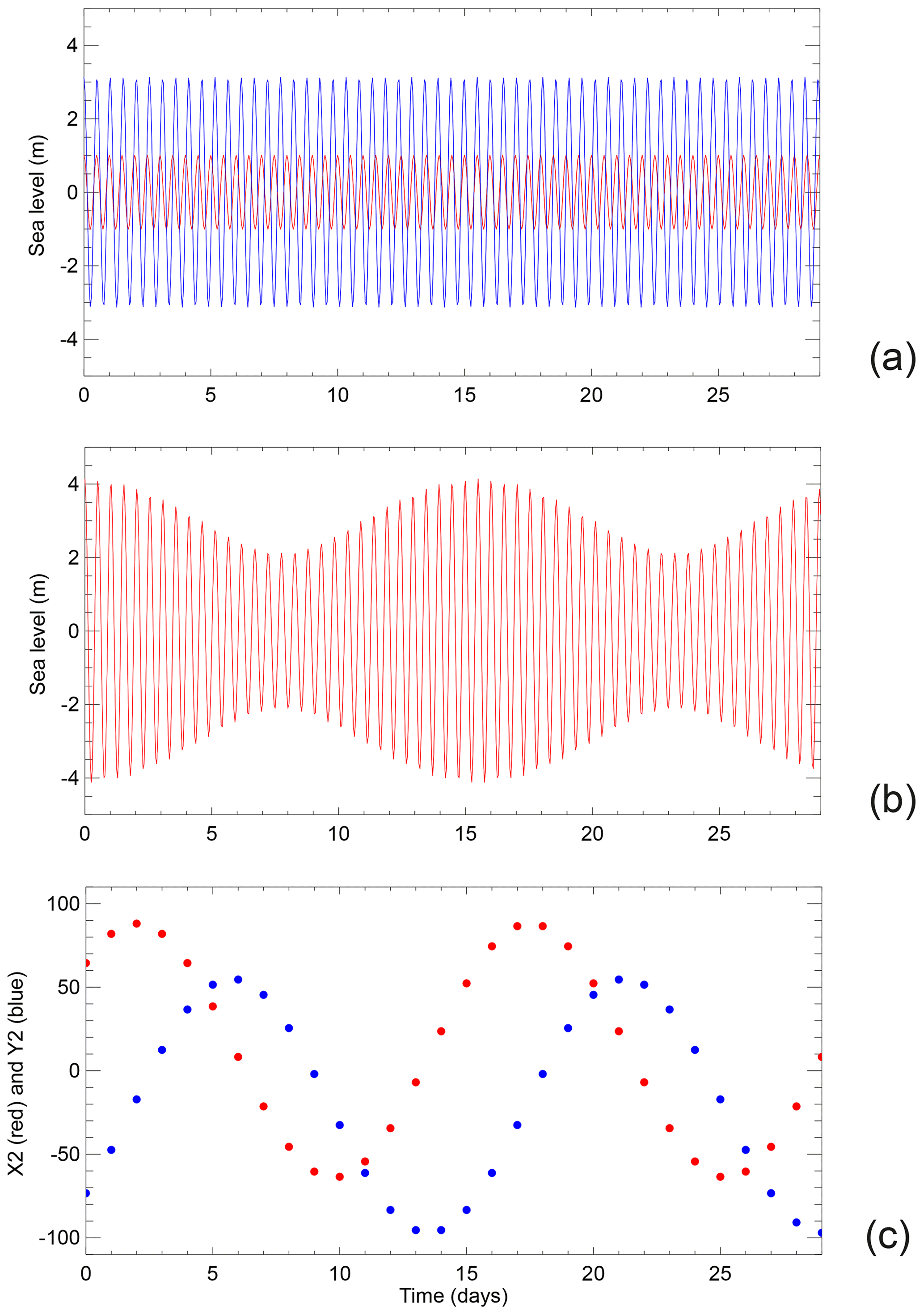
Figure 5(a) A schematic example of the variation of M2 (blue) and S2 (red) at Liverpool over a month, (b) M2 and S2 in combination and (c) the corresponding time series of daily values of X2 (red) and Y2 (blue).
Doodson's method of analysis of the hourly record made use of ingenious arithmetical filters designed to magnify the importance within the record of each constituent in turn, and so, after a lot of work, to arrive at a set of estimates of their amplitudes and phases. The multiplier coefficients of the various filters in effect functioned as a form of least-squares fit similar to the way constituents are determined in modern harmonic analysis. However, Doodson refused to be bound rigidly by the method of least squares, adopting it only as a guide to his own method. Consequently, multiplications by cosines and sines in the calculation of his coefficients were deemed to be unnecessary, with the cosines and sines, multiplied by 2, being replaced by the nearest integer (i.e. ±2, ±1 and 0). In addition, setting t=0 in the middle of the record simplified the calculations, as cosines were required to be multiplied only by cosines and sines only by sines. Furthermore, the method had some in-built redundancy, enabling a check on the quality of the computations and on the possibility of there being unexpected constituents in the record. The method is said to have revolutionised the analysis of tidal observations in many countries (Proudman, 1968). Normally 1 year of tide gauge data was adequate, with observations of the water level every hour, i.e. 8640 values in a 360 d year. (Doodson, 1954, described how shorter records may be analysed using similar methods.) His team of computers usually worked with values of water level in units of one tenth of a foot.
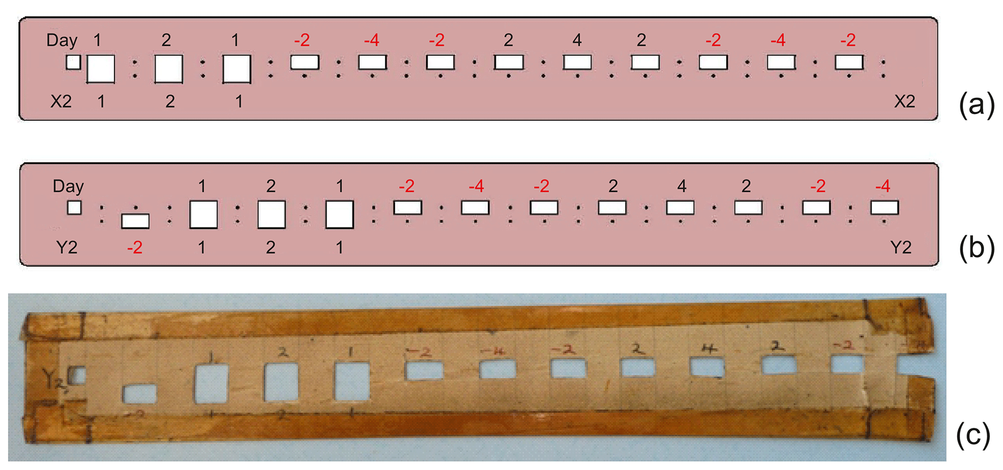
Figure 6(a) A schematic version of an original cardboard stencil for X2 with holes to show through those hours with data that had to be multiplied either by positive or negative weights. (b) A corresponding stencil for Y2. (c) An original cardboard stencil for Y2 showing the positive (black) and negative (red) weights. There were many pieces of cardboard like this for the different filters described in Doodson (1928). (Schematic versions courtesy of Ian Vassie.)
The method is described in detail in Doodson (1928) (see also Doodson and Warburg, 1941; Doodson, 1954). The work was labour intensive, involving endless arithmetic. However, Doodson claimed that an experienced computer could analyse the tabulated hourly heights to determine about 40 constituents in 10 working days of 6 h each, with 1 d for sundry checks by other computers. The analysis for 20 more constituents would take another 6 h.
In this method it was not necessary to manipulate all 8640 hourly water levels at once. 10 A first step involved the use of a set of filters to convert the hourly information into daily numbers, which have 24 times less the bulk of the original record. For the semi-diurnal constituents, these filters were called X2 and Y2 and were a set of simple integer arithmetic weights applied to the hourly values for each day. Other integer filters were designed for diurnal variations and other tidal components. 11
The computer listed on a page the hourly tide gauge values from hours 0 to 23 each day, with one line for each day, and then used a cardboard cut-out called a stencil, with holes for those hourly values which were to be multiplied by a filter weight for each hole. The spacing of values written on the page clearly had to be chosen so that the correct numbers would show through the appropriate holes in the stencil; suitable paper was especially printed for this purpose. The weight values themselves were written on the cardboard as shown schematically for the X2 filter in Fig. 6a.
The X2 filter for a particular day used data for hours 0–23 on that day and also hours 24–28 (i.e. hours 0–4 on the next day), spanning 29 h total. The integer weights were
The central value of the filter is shown underlined. The Y2 weights employed hours 3–23 on the required day and 24–31 on the next day and had the values
In this case the central value (shown underlined) is 3 h different from that of X2. Therefore, the two filters sample orthogonal components of the semi-diurnal variation. A schematic version of the Y2 stencil is shown in Fig. 6b and an original cardboard one in Fig. 6c. One can readily apply these filters to our example Liverpool data, and the daily time series of X2 and Y2 for Liverpool then appear as in Fig. 5c.
It can be seen that Fig. 5c has much the same information content as Fig. 5b (i.e. variation of the tide over a fortnight given two harmonic constituents) but with 24 times fewer numbers. The constant parts (the offsets) of the red and blue curves come from S2 because S2 is the same every day, while the cyclic parts, which vary over a fortnight, come from M2. Consequently, the red and blue offsets are a consequence of the amplitude and phase of S2, while the cyclic parts depend on the amplitude and phase of M2.12
However, it can be appreciated that this simple situation becomes more complicated when additional constituents are taken into account. For example, one can expect that S2, as it manifests itself in Fig. 5c for a particular month, will appear different in the next month if there is also significant K2 present in the record, and those differences will vary over half a year. In practice, M2 and S2 and all of the remaining semidiurnal constituents (such as 2N2, Mu2, N2, Nu2, Lambda2, L2, T2, R2 and K2) fall into “groups” according to the periods of their perturbation of X2 and Y2, with the group q perturbing X2 and Y2 by q complete periods per month. One can determine the magnitude of these perturbations for each group with a filter defined by another set of integer multipliers, one set of multipliers for each group. This yields a set of values denoted as, for example, X2q which refers to X2 after application of the multipliers for group q. This set X2q (and similarly Y2q) consists of 12 numbers, one for each month in the year.
Similarly, one will realise that each harmonic constituent within the group q will contribute to the set of 12 X2q values differently over a year. Consequently, by a suitable combination of X2q values, a quantity called X2qr can be obtained, where r signifies the number of periods of variation of X2q in the year. In general, a single X2qr (and Y2qr) corresponds to a particular harmonic constituent.
The first task of the computer was to calculate X2 and Y2 for each day, with the work done either by hand (which would take a considerable amount of time) or more usually later on with the use of a comptometer machine. She would then write the values for each day in a table with 12 columns (for 12 months of the year), with some columns having 29 rows and some having 30 rows. X2 (or Y2) values for days from the start to the end of the year (i.e. about 360 values) would be listed down column 1 first, then down column 2 etc. until the year was completed in column 12. Doodson (1928) called this exercise the “daily processes”.
The X2 (or Y2) values in each of the columns of the 12 months in this table were then multiplied by sets of integer weights for each group q. These were called “daily multipliers” (Table XV of Doodson, 1928), and this procedure was called the “monthly processes”. Then, the weighted X2 (or Y2) values in the 12 months of the year (denoted X2q and Y2q) were multiplied by further sets of integer weights for each month called “monthly multipliers” (Table XVI of Doodson, 1928) to provide X2qr (or Y2qr) values. These were called the “annual processes”.
As a consequence, these different sets of multipliers will have resulted in individual totalled quantities (X2qr or Y2qr) which, after a further “correction” stage for leakage into the X2qr and Y2qr from a small number of other constituents, will have magnified the importance of particular constituents within the record and so ultimately have provided an estimate of the constituent's amplitude and phase. For some constituents such as S2, estimates of amplitude and phase were given from the use of only certain multipliers (i.e. an individual 2qr), but for others, such as K2, they were provided through the use of more than one 2qr, requiring combination in an additional stage.
Finally, because the analysis set t=0 in the middle of the 1-year record, there was a need to adjust the derived amplitudes and phases for the appropriate astronomical arguments and nodal factors at that time. These could be computed using standard formulae.
It can be seen that this was a complicated and labour intensive procedure, but it was straightforward once it could be explained clearly to a computer with basic mathematical skills equipped with one of the mechanical or electronic calculating machines available at that time. The method is described in detail in Doodson (1928) with a worked example for a year of data from Vancouver 13.
Doodson (1928) explained that his was not the first such method. There were many papers published in the 19th century which list amplitudes and phases for harmonic constituents computed in different ways (e.g. see Baird and Darwin, 1885). Most of these will have used the method devised by Thomson, Roberts and Darwin and published in BAAS reports between 1866 and 1885 (e.g. Darwin, 1884). This was the method employed by Roberts and the Survey of India to determine amplitudes and phases for use with their TPMs.14 There was also Darwin's later method (Darwin, 1893), of which Doodson (1928) claimed his to be a further development. There was a popular method invented in Germany by Börgen (1894) which was studied for use in several countries (e.g. Adams, 1910). The US Coast and Geodetic Survey also had its own method based on the intensive use of many filters (USCGS, 1894). Doodson (1928) provides a short discussion of the relative merits of each method. They were said to differ in the amount of labour involved (the BAAS method was said to require the most labour; Börgen's method required the least until Doodson's became available); in how well they could eliminate the overlap of information from different constituents in the derivation of the amplitudes and phases; and in the completeness of the analysis. However, so far as I know, there was never a detailed, quantitative comparison between methods. 15
Doodson then had all the amplitudes and phases that he needed to set up his TPM, including those of the semidiurnal, diurnal, shallow-water and long-period tides calculated by similar filtering to that described above. All the amplitudes and phases were written on a special “running card” for the port in question and for the year requiring prediction by the machine. These values were derived from “constants cards”, which contained a list of amplitudes and phase lags for the particular port and from values of V, f and u for the year in question, as explained below. Each “running” (or “setting-up”) card was colour coded according to the particular year. Figure 7a and b shows the front and reverse of a relatively recent example of a card that was used for operation of the Bidston Doodson–Légé Machine (TPM-S20). Those used earlier for the Doodson–Légé Machine and the two other Bidston machines will have been similar.16
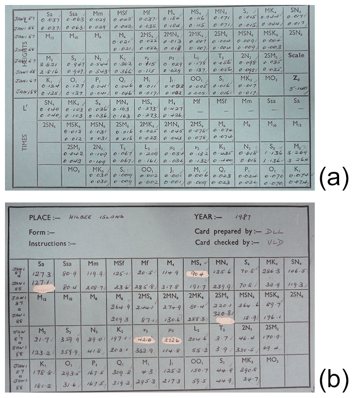
Figure 7(a, b) The two sides of a relatively recent “running card” for use with the Bidston Doodson–Légé Machine, in this case for producing predictions for Hilbre Island in 1987 and 1988. (Card courtesy of Valerie Gane.)
The top part of one side of the card (Fig. 7a) shows values for f times amplitude for each constituent, in the order that the constituents appear on the front of the machine, for Hilbre Island (near Liverpool) for 1 January 1987 and 1988. The values are in metres, and the lunar ones such as M2 are slightly different for the 2 years because their nodal factors f vary from year to year (Pugh and Woodworth, 2014). In fact, January 1988 was close to a nodal minimum for M2. The values for the solar constituents such as S2 are the same for both years. The lower part of the card shows the values of (frequency × amplitude) for each year, with an overall scaling factor for the Doodson–Légé Machine, which represents the rate of change of the constituent (i.e. Eq. 2).17
These amplitude values are set using the shafts (also called “amplitude blocks”) for each wheel on the front of the machine using a Vernier screw, and the corresponding values (frequency × amplitude) are set similarly on the back of the machine. As explained above, the machine is a double-sided one, in effect two separate machines, with one side calculating the instantaneous height of tide level and the other the rate of change of level. Finally, the phases for each constituent, shown on the reverse of the card for each year (Fig. 7b), are set using the wheels at the front of the machine using the rotating dials. (In order to rotate the dials, it is first necessary to release the associated clutch, remembering to tighten it up again before running the machine, otherwise the contribution of the particular constituent would not be included in the total tide.) These phases are not phase lags (or they would be the same for both years) but are values of , where V is the astronomical argument for the start of the year in question, u is its nodal correction and g is the Greenwich phase lag for that constituent. All of these values can all be computed readily for any year, once one has calculated h and g as explained in Sect. 6.
Setting up the Doodson–Légé Machine in this way by an experienced person requires approximately an hour, after which the settings should be checked by another computer. It then takes an operator 1 or 2 d to produce a complete set of high and low waters for any given year. The LTI procedure then required a junior computer to undertake a step called “differencing” in which each day's predicted high- and low-water heights and times were subtracted from those of the next day. Then, a more senior computer performed a “smoothing” step to check that the differences contained no unexpected errors, plotting out the differences if necessary. Any errors resulted in an iteration of differencing and smoothing. Finally, a step called “writing up” prepared the results for a customer. Schofield (2006) states that the whole process of producing a year's predictions for a single port took about 4 d, involving several people and about 30 man-hours of work.
A team of computers such as that at the LTI could produce many sets of predictions every year with the use of the TPMs. Scoffield (2006) states that by 1944 the LTI was the foremost tidal predicting institute in the world, providing three times the quantity of predictions as the US Coast and Geodetic Survey. By the mid-1950s, the use of the Doodson–Légé TPM enabled predictions to be produced under contract for up to 180 ports worldwide annually (Cartwright, 1999). These predictions were made available to many important customers including the Admiralty; Scoffield (2006) also remarks that at this time the LTI was supplying over 600 sets of predictions annually for use in almanacs.18 As a result, they provided an important source of income to the LTI over many years, as discussed by Carlsson-Hyslop (2010).
Of course, tidal predictions can be made nowadays in a fraction of a second using a modern digital computer. 19 However, speed is not the major consideration, but it is rather the expertise of the person or team making such calculations. It was satisfying to find in a recent test that the Doodson–Légé Machine, recently refurbished by National Museums Liverpool, provided high- and low-water predicted heights and times for Liverpool for 2016 that were very similar to those produced by modern tidal software.
This paper has discussed how TPMs came to be invented at the end of the 19th century and were manufactured in reasonable numbers in the first half of the 20th century. It is gratifying that most of the 30 or so constructed around the world still survive and are on public display, even if they are not in full working condition. The paper has also provided a schematic description of how they worked. However, we have a lot to learn about the detailed design of individual machines. Although many of them were made by the same manufacturer, they were all different in some respects, probably due to it being thought desirable to make “improvements” each time. After the passage of time, some details are hard to understand without the most complete original engineering drawings and archives of correspondence and without the time to fully research them. Therefore, there is scope for much further investigation into them.
In addition, the paper has demonstrated the importance of the TPMs during the first half of the 20th century in providing tidal predictions for both scientific and practical applications. In particular, it has been shown that the LTI and Arthur Doodson played a central role in this area of research between the 1920s and 1960s, after which the advent of digital computers consigned most of these interesting machines to museums. It is fitting that the 100th anniversary of the LTI (now part of the UK National Oceanography Centre; NOC), coinciding with the anniversary of the founding of the first oceanography department in the UK at Liverpool University and of the IUGG, is being celebrated by the various papers on tides in this special issue. And it is important that the work with the TPMs by Doodson and others be recognised within that overall history.
No data sets were used in this article.
Some of this paper is based on unpublished reports by PLW including the inventory of Woodworth (2016) and occasional contributions to the website of Bidston Observatory (http://bidstonobservatory.org.uk, last access: 16 March 2020).
The author declares that there is no conflict of interest.
This article is part of the special issue “Developments in the science and history of tides (OS/ACP/HGSS/NPG/SE inter-journal SI)”. It is not associated with a conference.
I am grateful to several former employees of NOC for information on the methods of tidal analysis and prediction at the LTI, including the use of the TPMs. They include Ian Vassie, Sylvia Asquith, Valerie Gane (formerly Valerie Doodson) and Joyce Scoffield. And I thank David Cartwright, David Pugh, Trevor Baker and others at Bidston Observatory for whatever I know about tides in general. Steve Newman and others at National Museums Liverpool are thanked for their recent excellent refurbishments of the Roberts–Légé and Bidston Doodson–Légé machines (TPM-S5 and TPM-S20), a project which taught us a lot about TPMs. Also I thank Paul Hughes, formerly of Liverpool John Moores University, Nicolas Pouvreau of SHOM, France, for communications about the history of TPMs, and Helen Rawsthorne of the Université de Bretagne Occidentale, whose recent master's thesis provided further insights into them. Valerie Gane, Joyce Scoffield, Helen Rawsthorne and Liz Bradshaw of NOC provided valuable comments on drafts of the paper. In addition, I thank David Bowers and Marie-José Durand-Richard for their valuable comments.
This paper was edited by Mattias Green and reviewed by David Bowers and Marie-José Durand-Richard.
Adams, C. E.: The harmonic analysis of tidal observations, in: Proceedings of the Wellington Philosophical Society, Sixth Annual General Meeting, 5 October 1910, 83–84, 1910.
Baird, A. W. and Darwin, G. H.: Results of the harmonic analysis of tidal observations, Philos. T. R. Soc., 39, 135–207, https://doi.org/10.1098/rspl.1885.0009, 1885.
Bashforth, F.: Tide-predicting machines, Nature, 24, 53–53, https://doi.org/10.1038/024053b0, 1881.
Börgen, C.: Über eine neue methode, die harmonischen konstanten der gezeiten abzuleiten, Annalen der Hydrographie und Maritimen Meteorologie, 220, 256–270, 1894.
Carlsson-Hyslop, A.: Human computing practices and patronage: antiaircraft ballistics and tidal calcuations in First World War Britain, Inform. Cult., 50, 70–109, https://doi.org/10.1353/lac.2015.0004, 2015.
Carlsson-Hyslop, A. E.: An anatomy of storm surge science at Liverpool Tidal Institute 1919–1959: forecasting, practices of calculation and patronage, PhD thesis, University of Manchester, 306 pp., 2010.
Carlsson-Hyslop, A. E.: How the Liverpool Tidal Institute was established: industry, navy and academia, Hist. Geo Space. Sci., submitted, 2020.
Cartwright, D. E.: The historical development of tidal science, and the Liverpool Tidal Institute, in: Oceanography of the Past, edited by: Sears, M. and Merriman, D., New York, Springer-Verlag, 812 pp., 240–251, 1980.
Cartwright, D. E.: Tides: a scientific history, Cambridge, Cambridge University Press, 292 pp., 1999.
Darwin, G. H.: Report of a committee for the harmonic analysis of tidal observations, Report of the 53rd Meeting of the British Association for the Advancement of Science held in Southport in September 1883, London, Charles Murray, 49–117, 1884.
Darwin, G. H.: I. On an apparatus for facilitating the reduction of tidal observations, Proc. Roy. Soc., 52, 345–388, https://doi.org/10.1098/rspl.1892.0082, 1893.
De Mol, L. and Durand-Richard, M. J.: Calculating machines and numerical tables – a reciprocal history, available at: http://hal.univ-lille3.fr/hal-01396846 (last access: 16 March 2020), 2016.
Doodson, A. T.: The tides and the work of the Tidal Institute, Liverpool, Geogr. J., 63, 134–144, available at: http://www.jstor.org/stable/1781626 (last access: 16 March 2020), 1924.
Doodson, A. T.: The machine which works with the Moon. Predicting the rise and fall of the tides, The Graphic Magazine, 14 March 1925, p. 401, 1925.
Doodson, A. T.: Tide-predicting machines, Nature, 118, 787–788, https://doi.org/10.1038/118787a0, 1926.
Doodson, A. T.: How science aids port navigation – Liverpool and tidal research, Mersey Magazine, Vol. 5, 1927 (reprinted in 293–296; chap. 17 of Scoffield 2006).
Doodson, A. T.: The analysis of tidal observations, Philos. T. R. Soc. A, 227, 223–279, https://doi.org/10.1098/rsta.1928.0006, 1928.
Doodson, A. T.: New tide-prediction machines, Int. Hydrogr. Rev., 28, 88–91, 1951.
Doodson, A. T.: The analysis of tidal observations for 29 days, Int. Hydrogr. Rev., 31, 3–31, 1954.
Doodson, A. T.: The analysis and prediction of tides in shallow water, Int. Hydrogr. Rev., 34, 85–126, 1957.
Doodson, A. T. and Warburg, H. D.: Admiralty manual of tides, London, His Majesty's Stationery Office, 270 pp., 1941.
Durand-Richard, M.-J.: De la prédiction des marées: entre calcul, observations et mécanisation (1831–1876), Cahiers François Viète, série II, 8/9, 105–135, 2016a.
Durand-Richard, M.-J.: Historiographie du calcul graphique, available at: https://halshs.archives-ouvertes.fr/halshs-01516382 (last access: 16 March 2020), 2016b.
Hicks, S. D.: The tide prediction centenary of the United States Coast and Geodetic Survey, Int. Hydrogr. Rev., 44, 121–131, 1967.
Hughes, P.: A study in the development of primitive and modern tide tables, PhD thesis, Liverpool John Moores University, 340 pp., 2005.
IHB: Tide predicting machines, International Hydrographic Bureau Special Publication No. 13, Monaco, International Hydrographic Bureau, 110 pp., 1926.
Joselyn, J. A. and Ismail-Zadeh, A.: Preface to the special issue “The International Union of Geodesy and Geophysics: from different spheres to a common globe”, Hist. Geo Space. Sci., 10, 17–24, https://doi.org/10.5194/hgss-10-17-2019, 2019.
LDP: Liverpool Daily Post newspaper for Tuesday 25 July, p. 2, 1944.
Lubbock, J. W.: Discussion of tide observations made at Liverpool, Philos. T. R. Soc., 125, 275–299, https://doi.org/10.1098/rstl.1835.0017, 1835.
MacLennan, B. J.: Analog computation, in: Unconventional Computing, edited by: Adamatzky, A., New York, Springer, 693 pp., 3–33, 2018.
Nature: Liverpool Observatory and Tidal Institute (Nature News Item), Nature, 122, 979–980, https://doi.org/10.1038/122979b0, 1928.
NOAA: Web site of the National Oceanic and Atmospheric Administration, History of Tidal Analysis and Prediction, available at: https://tidesandcurrents.noaa.gov/predhist.html, last access: 1 September 2019.
Parker, B.: The tide predictions for D-Day, Phys. Today, 64, 35–40, https://doi.org/10.1063/PT.3.1257, 2011.
Proudman, J.: Report on harmonic analysis of tidal observations in the British Empire, in: British Association for the Advancement of Science Report of the 88th Meeting, London, 323–345, 1920.
Proudman, J.: Arthur Thomas Doodson, 1890–1968, Biographical Memoirs of Fellows of the Royal Society, 14, 189–205, https://doi.org/10.1098/rsbm.1968.0008, 1968.
Proudman, J. and Doodson, A. T.: The principal constituent of the tides of the North Sea, Philos. T. R. Soc. A, 224, 185–219, https://doi.org/10.1098/rsta.1924.0005, 1924.
Pugh, D. T. and Woodworth, P. L.: Sea-level science: Understanding tides, surges, tsunamis and mean sea-level changes, Cambridge, Cambridge University Press, 408 pp., 2014.
Qi, S.: Use of International Hydrographic Organization tidal data for improved tidal prediction, Portland State University Master's thesis, Dissertations and Theses, Paper 900, 2012.
Rawsthorne, H. M.: An historic analysis of tide prediction machines using an adapted prosopographic approach and digital humanities tools, Master's Thesis, Université de Bretagne Occidentale, 48 pp., https://doi.org/10.5281/zenodo.3265011, 2019.
Rossiter, J. R.: The history of tidal predictions in the United Kingdom before the twentieth century, Proc. R. Soc. Edinb. B, 73, 13–23, https://doi.org/10.1017/S0080455X00002071, 1971.
Sager, G.: Gezeitenvoraussagen und Gezeitenrechenmaschinen, Warnemünde: Seehydrographischer Dienst der Deutschen Demokratischen Republik, 126 pp., 1955.
Scoffield, J.: Bidston Observatory: the place and the people, Merseyside, Countryvise Ltd., 344 pp., 2006.
SHOM: Tidal predictor (SHOM web site), available at: http://www.shom.fr/en/activities/activites-scientifiques/maree-et-courants/marees/predicteur-de-maree, last access: 1 September 2019.
Thomson, W.: IV. Harmonic analyser, Proc. R. Soc., 27, 371–373, https://doi.org/10.1098/rspl.1878.0062, 1878.
Thomson, W.: The tide gauge, tidal harmonic analyser, and tide predictor, Proc. Inst. Civil Eng., 65, 2–25, https://doi.org/10.1680/imotp.1881.22262, 1881.
Thomson, W.: The tides. Evening lecture to the British Association at the Southampton Meeting on Friday, 25 August, in: Popular Lectures and Addresses, Vol. III, Navigational Affairs, London, Macmillan and Co., 1891, 139–190, available at: https://archive.org (last access: 16 March 2020), 1882.
Thomson, W. and Tait, P. G.: Treatise on natural philosophy, Part 1 (reprinted 1912), Cambridge, Cambridge University Press, 508 pp., 1879.
Tide and Time: Tide and time web site, available at: https://www.tide-and-time.uk/tide-predicting-machines, last access: 1 September 2019.
USCGS: Report of the Tidal Division of the U.S. Coast and Geodetic Survey Office for the Fiscal Year ending 30 June, 1893, 107–109, in: Report of the Superintendent of the U.S. Coast and Geodetic Survey showing the progress of the Work during the Fiscal Year Ending with June 1893, Part I. Washington: Government Printing Office, 167 pp., available at: https://library.noaa.gov/Collections/Digital-Collections/USCGS-Annual-Reports (last access: 16 March 2020), 1894.
USCGS: Description of the US Coast and Geodetic Survey Tide-Predicting machine no. 2, US Coast and Geodetic Survey Special Publication No. 32, Washington D.C., Department Of Commerce, available at: https://library.noaa.gov/Collections/Digital-Collections/USCGS-Special-Pubs (last access: 16 March 2020), 1915.
Webb, E. K. and Bacon, N. E.: A mechanical harmonic analyser, J. Sci. Instrum., 39, 500–503, https://doi.org/10.1088/0950-7671/39/10/303, 1962.
Whewell, W.: Essay towards a first approximation to a map of cotidal Lines, Philos. T. R. Soc., 123, 147–236, https://doi.org/10.1098/rstl.1833.0013, 1833.
Woodworth, P. L.: An inventory of tide prediction machines, National Oceanography Centre Research and Consultancy Report No. 56, Southampton, National Oceanography Centre, 71 pp., available at: http://nora.nerc.ac.uk/513660/ (last access: 16 March 2020), 2016.
Equation (1) is shown in a simplified form, omitting astronomical arguments and nodal factors and with the mean level set to zero. It can be written more fully as , where Vi is called the astronomical argument for constituent i at time t=0 and the nodal factors fi and ui are time-dependent adjustments to the amplitudes and phase lags respectively of lunar tidal constituents (those for solar constituents are simply 1.0 and 0.0 respectively); V, f and u can all be computed readily using standard formulae which are derived from knowledge of the orbits of the sun and moon; and Z0 indicates the mean level of the record. See Pugh and Woodworth (2014) for more details.
The idea for TPMs was clearly not Kelvin's alone. For example, the Rev. Francis Bashforth explained in 1881 how he had had an idea for a four-component machine in 1845 (Bashforth, 1881; IHB, 1926; Hughes, 2005).
The two sides of the machine were known at the LTI as the times and heights sides, rather than the rates and heights sides. The LTI names referred to the intended application, which was to compute the times and heights of high and low waters. Two dials can be seen on the left-hand side of the front of the machine beneath the paper chart cylinder and above a panel showing the date and time (Fig. 3f). The left-hand dial displays the rates (or “gradients” as Doodson, 1951, referred to them), for use either when the original single-sided machine was set up to provide Eq. (2) or now using the times (back) side of the present double-sided machine. The right-hand dial displays the heights, for use either when the original machine was set up for Eq. (1) or now using the heights (front) side of the present machine.
An even earlier list of the small number of machines in existence at the time was given in USCGS (1915).
Doodson had also evidently been in contact with the Hydrographic Department of the Chinese navy concerning the acquisition of a machine. A letter from the navy to Doodson in December 1947 stated that they had ordered one from Marine Instruments Ltd. (i.e. KBB). However, there is no evidence that such a machine was delivered. Much earlier, Doodson had heard from KBB in 1931 that they had been approached about a machine for China, but nothing seems to have come of that either.
Schoffield (2006) mentions that the initial estimate by Légé was GBP 4150 for a single-sided machine that could be upgraded as funding permitted.
There were some 5000 gear ratios involved in the design of the Bidston Doodson–Légé Machine.
The 11 components were designed to determine the five tidal constituents M2, S2, K1, O1 and P1 (i.e. h cos (g) and h sin (g) for each) plus the mean water level. Proudman (1920) states that the five constituents included M4 instead of P1, although that is not supported by Thomson (1881, 1882) or the surviving Science Museum documentation.
A good impression of the working relationships between Doodson and his team of computers and other staff at Bidston Observatory is given by Scoffield (2006).
Darwin (1893) had adopted a similar necessary approach of reducing the size of tidal data sets to manageable proportions.
The way that the X2 filter was selected is described in Sect. 5 of Doodson (1928). He remarked that “it is unnecessary to illustrate the genesis of the remaining formulae”.
The sums of the weights of X2 and Y2 are zero, so changes in mean sea level do not contribute to the offsets for S2.
However, this is not a complete worked example, and there are some errors e.g. p. 258 and Table XXX of Doodson (1928) refer to a datum value of 500 for X2, Y2 which should be 600.
The India Office Machine was used to make the tidal predictions for India and elsewhere, although it was located first in England for over 40 years, first at Lambeth and then at the National Physical Laboratory in Teddington, until it was moved in 1921 to the headquarters of the Survey of India in Dehra Dun.
Tidal constants from many coastal locations produced by the LTI and other national tidal agencies would eventually form the basis of the International Hydrographic Organization tidal databank (Qi, 2012). In turn, the databank would aid the development of regional and global tidal charts and tide models. The construction of tidal charts had been an important research topic since the middle of the 19th century (e.g. Whewell, 1833) and was one in which Doodson himself had been engaged in the early years of the LTI (Proudman and Doodson, 1924; Cartwright, 1999).
Most running cards were colour-coded and contained information for only 1 year. However, the values for the 2 years shown in this particular example are useful in demonstrating the nodal dependence of the lunar constituents.
There were also running cards which contained values corresponding to times during the year additional to 1 January (e.g. 1 April and 1 October). This enabled the machine to be run several times for each year with the resulting sets of predicted heights and times of high and low waters checked for consistency.
The written-up sets of predictions were reproduced photographically before delivery to customers. Copies were also kept for future reference. In the case of major ports, the writing up involved typing values using specially configured typewriters with continuous carbon tape instead of ribbons, so as to obtain perfectly sharp characters for direct photo-lithographic reproduction in the Admiralty Tide Tables.
Proudman (1968) (see also Cartwright, 1999) remarked that towards the end of Doodson's tenure as LTI director he strenuously opposed the use of modern digital computers, claiming that they would increase the cost of providing tidal predictions to harbour authorities. That reservation is understandable given Doodson's lifetime involvement with the TPMs and the fact that they were still a source of income. It was left to his successor (Jack Rossiter) to introduce modern computers to the LTI, where they were used extensively for research into tides and storm surges.
- Abstract
- Introduction
- The harmonic method
- Schematic description of a TPM
- TPM inventory
- The three TPMs at the LTI
- The required harmonic constants
- Setting up the TPM
- Conclusions
- Data availability
- Author contributions
- Competing interests
- Special issue statement
- Acknowledgements
- Review statement
- References