the Creative Commons Attribution 4.0 License.
the Creative Commons Attribution 4.0 License.
 | 05 Jun 2019
Auroral hydrogen emissions: a historic survey
Alv Egeland
William J. Burke
Auroral spectroscopy provided the first tool for remotely sensing the compositions and dynamics of the high-latitude ionosphere. In 1885, Balmer discovered that the visible hydrogen spectrum consists of a series of discrete lines whose wavelengths follow a simple mathematical pattern, which ranks among the first steps toward developing this tool. On 18 October 1939 Lars Vegard discovered the Hα (656.3 nm) and Hβ (486.1 nm) spectral lines of Balmer series emissions, emanating from a diffuse structure, located equatorward of the auroral zone. Intense, first positive bands of nearly covered the Hα emissions.
With more advanced instrumentation after World War II, auroral spectroscopists Vegard, Gartlein and Meinel investigated other characteristics of the auroral hydrogen emissions. The first three lines of the Balmer series, including Hγ at 410 nm, were identified in ground-based measurements prior to the space age. Based on satellite observations, the Balmer lines Hδ and Hε at 410.13 and 396.97 nm, respectively, as well as extreme ultraviolet (EUV) Lyman α (121.6 nm) hydrogen emissions, were also detected.
Doppler blue shifts in hydrogen emissions, established in the 1940s, indicated that emitting particles had energies well into the kiloelectron volt range, corresponding to velocities >1000 km s−1. Systematic spatial separations between the locations of electron- and proton-generated aurorae were also established. These observations in turn, suggested that protons, ultimately of solar origin, precipitate into the topside ionosphere, where they undergo charge-exchange events with atmospheric neutrals. Newly generated hydrogen atoms were left in excited states and emitted the observed Balmer radiation. Sounding rocket data showed that most of the hydrogen radiation came from altitudes between 105 and 120 km.
Space-age data from satellite-borne sensors made two significant contributions: (1) energetic particle detectors demonstrated the existence of regions in the magnetosphere, conjugate to nightside proton aurora, where conditions for breaking the first adiabatic invariants of kiloelectron volt protons prevail, allowing them to precipitate through filled loss cones. (2) EUV imagers showed that dayside hydrogen emissions appear in response to changes in solar wind dynamic pressure or the polarity of the north–south component of the interplanetary magnetic field.
- Article
(1762 KB) - Full-text XML
- BibTeX
- EndNote


Pioneering spectroscopic work by Anders Ångstrøm (1814–1874) in the 1850s marks the beginning of quantitative spectral studies as applied to the northern lights. Ångstrøm (1868) used a theodolite with a transmission grating when discovering the auroral green line at 5578 angstrom (Å). Thereby he introduced the wavelength unit, cm, which appeared well suited to optical spectroscopy. Today the unit of preference is nanometers (nm), where 1 nm=10 Å. In 1960, 1 Å was defined officially as being equal to 10−10 m (Franke, 1969).
In 1906 Lars Vegard (1880–1963), a central character of the present narrative, began to work as an assistant to professor Kristian Birkeland (1867–1917). Subsequent to Birkeland's death, Vegard was appointed professor of physics at the University of Kristiania (now Oslo) in 1918. He soon developed a high-quality scientific laboratory at the university. Around 1920 he devised a double-prism spectrograph with resolution sufficient to specify the auroral green line's accurate to the wavelength 557.7±0.1 nm (Vegard, 1923; Babcock, 1923). He is widely known for identifying several auroral emissions associated with atmospheric nitrogen (Vegard, 1956). Vegard also contributed to the development of competing excitation models proposed to explain the generation of the auroral green line emissions. This spectral line was not reproducible in a laboratory until 1924 (McLennan and Shrum, 1925). During the period 1950–2000, numerous papers discussed different indirect excitation mechanisms other than transitions between O(1S) and O(1D) atomic states (Omholt, 1971; Vallance Jones, 1974). This review concentrates on hydrogen emissions excited by energetic protons bombarding the auroral ionosphere.
In 1908 and 1912, Vegard conducted advanced spectroscopic studies at Cambridge and Würzburg universities under the direction of Professors Joseph Jon Thomson and Wilhelm Wien, respectively. He wished to study emissions generated by cathode and anode rays for comparison with auroral spectral lines. During this time, he was assembling arguments in support of his hypothesis that the aurora could be produced by energetic helium ions (alpha rays) bombarding the upper atmosphere (Vegard, 1911). The title of his 1911 paper in Nature was “The Radiation Producing Aurora Borealis”. At this time, the only known sources of energetic particles were radioactivity and cathode rays.
Auroral scientists Kristian Birkeland and Carl Størmer (1874–1957) strongly influenced Vegard's research. As a young man, he worked closely with Birkeland. Later he came to admire Størmer's calculations of auroral particle orbits that simulated Birkeland's Terrella experiments (Egeland and Burke, 2012). In 1896, Birkeland offered a radically new perspective on the auroral problem, suggesting that cathode rays from the Sun excited the emissions (Egeland and Burke, 2005). This occurred 3 years before J. J. Thomsen first identified electrons as current-carrying particles. In a 1952 paper, Vegard wrote “I suggested (both in 1916 and 1928) that the bundles of solar electric rays produce aurorae and that most magnetic disturbances are composed of electrons, electrostatically neutralized by positive ions of great specific charge, mainly protons.” Thus, Vegard was arguing that the solar electrons must be accompanied by protons. If not, powerful polarization electric fields would halt electron precipitation (Schuster, 1911). Vegard, however, was first to suggest that positive ions must accompany solar electrons. Later investigations (Vegard, 1948; Omholt, 1971) realized that He lines due to precipitating α-particles are also observed, but only rarely, in the aurora spectra.
In 1885 the Swiss physicist Jakob J. Balmer (1825–1898) observed that wavelengths of visible spectral lines of hydrogen were well ordered, in what is now referred to as the Balmer series. Bohr (1913) explained his simple formula as representing the wavelengths of visible H emissions that reflect the discrete energy states available to hydrogen atoms.
Starting in 1927, Vegard operated spectrographs at both The Auroral Observatory in Tromsø (geographic coordinates 69∘26′′ N, 18∘54′′ E; geomagnetic latitude 67.1∘ N) and near the University of Oslo, about 10∘ in magnetic latitude to the south. Simultaneous measurements at two separated sites documented auroral emission variations with latitude and altitude. It was during these observations that he discovered the Vegard–Kaplan band system (Egeland and Burke, 2016).
Vegard's most famous auroral-spectroscopic discovery occurred on 18 October 1939 (see Fig. 1), when he detected the two spectral lines of the Balmer series, Hα (656.3 nm) and Hβ (486.1 nm), in northern lights in a diffuse cloud-like aurora, equatorward of the auroral zone. The Hα emissions was nearly covered by the strong first positive bands of and the intensity was about one-fifth of the oxygen green line at 577.7 nm (Vegard, 1939). The Hβ line was close to one of the N2 Vegard–Kaplan bands. Photographic observations by Størmer showed that this auroral event – in southern Norway – persisted for many hours. These hydrogen emissions were observed, using low-dispersion spectrographs, within a quiet, diffuse, evening-sector, auroral arc, on the equatorward side of a form over Oslo. Surprisingly, these lines had not appeared in similar observations made in prior years (Vegard, 1939).
A total of 3 months after his first publication on hydrogen lines, Vegard published a second paper titled “On some recently detected important variations within the auroral spectrum”, in the March 1940 issue in the journal Terr. Magn. Atmos. Elect. There he stated
the simultaneous enhancements of two lines, one coincides with the Hα the other with Hβ, can hardly be accidental, and our spectrograms thus would give evidence of a situation where considerable quantities of hydrogen was present in the auroral region. The numerous spectrograms obtained during earlier years, when the hydrogen lines are absent, indicate that noticeable quantities of hydrogen are rarely found. Thus, the occurrence of these H lines must be due to showers of hydrogen to a kind of `hydrogen radiation' occasionally coming from the Sun.
Later, Vegard and Tønsberg (1941) demonstrated the detection of the Hγ line (410 nm) at the Auroral Observatory in Tromsø, based on data from the most reliable sensors available prior to the space age. Neither Doppler broadenings nor shifts were reported in early measurements.
In 1952, Vegard published a new paper on proton aurora, in which he wrote
in 1939, I took a series of auroral spectrograms, in which hydrogen showed a powerful spectroscopic line. In the winter 1940–1941, we were able to make a series of spectrograms using a sensor that had considerably more resolution than the one in Oslo. In some of the Tromsø spectrograms, the hydrogens lines assumed the shapes of narrow bands that were strongly deflected towards the shorter wavelengths. This could only mean that emitting hydrogen atoms, were moving quickly towards the ground.
Vegard later found hydrogen lines in spectra taken at the Tromsø Observatory in 1940 and the following years. Since occurrences of proton aurora were sporadic, he concluded that hydrogen cannot be an important atmospheric constituent. Rather, they reflect “hydrogen showers from the Sun.” The much greater dispersion of the Tromsø spectrograph demonstrated that the Hβ line was much more clearly identifiable than during earlier observations. Another reason why Hα, the strongest visible hydrogen line, had not been detected previously is that it is often embedded within intense first positive bands of emissions. Consequently, they were unresolvable with then available spectroscopic technologies.
In the years shortly after Vegard's first two papers, auroral scientists began to pay greater attention to recently detected hydrogen emissions, and confirmed that occurrences were sporadic. On 3 January 1940, Størmer (1955) detected two hydrogen lines over Oslo at altitudes near 110 km. In 1942, C. W. Gartlein observed H emissions in aurora above New York state, equatorward of Oslo's magnetic latitude. He also noted that emissions were spectrally broadened, but not shifted. As the Hβ line was much broader than other lines, Gartlein (1950) first assumed that it could not be an atomic line. Consistent with Vegard's results, Gartlein later concluded that hydrogen is not an upper atmosphere constituent. Rather, the auroral emissions must result from proton “showers” of solar origin.
According to the international literature, Vegard (1950) was first to observe Doppler-shifted Hβ line emissions on 23 February 1950 as discussed in his paper in Nature. There he presented shifts toward the violet portion of the visible spectrum, indicating that the responsible H atoms were incoming at high speeds. However, in a report presented at a meeting in Brussels on 28–30 July 1948, Vegard wrote
on spectrograms with the greatest dispersions, the sharp Hβ line vanished, but in its place there appeared at shorter wavelengths, a broad band or a line at 485.65 nm. This fact suggests that we were observing the Hβ line, displaced via the Doppler effect. Average displacements were about 0.5 nm, corresponding to mean velocities of ∼300 km s−1 towards the observer (Vegard, 1948).
Similar observations were also presented at the IUGG Conference of Oslo Meeting, 19–28 August 1948 (Joyce, 1950; Omholt, 1971). Here he mentioned broadened Hβ lines observed near the horizon and Doppler shifts towards shorter wavelengths near zenith.
Characteristic of proton aurora, both significant Doppler broadening and shifting of the lines occur. Prior to the early 1940s, such details were undetectable. However, during solar cycle 18 the level of geomagnetic activity rose significantly. Figure 2 provides an example of proton-emission spectra recorded at the Oslo (Fig. 2a) and Tromsø (Fig. 2b) observatories. They illustrate spectral differences obtained when an observer looks along the field line toward local zenith versus looking perpendicular to the field at auroral heights. In a later paper, Fig. 3 from Vegard (1952) provides an enlarged copy of a photometer trace acquired at Tromsø in October 1941. The marked shift of the Hβ line corresponds to an incoming H speed of 1970 km s−1. Still larger shifts have been observed. For the sake of comparison, the lower trace exemplifies the Hβ line with no displacement.
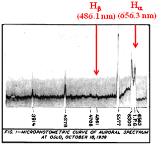
Figure 1Vegard's first spectrum illustrating the presence of hydrogen emissions from an aurora, recorded at the University of Oslo on 18 October 1939.
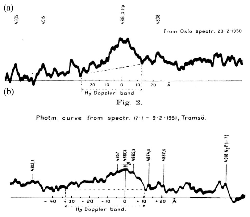
Figure 2This figure shows hydrogen northern-light emissions, observed about a year apart, at Oslo (a) and Tromsø (b).
The nearly symmetric curve from Oslo (lower curve in Fig. 3) exemplifies the unshifted Hβ line. Figure 4 schematically illustrates the situation as simultaneously viewed by two observers. The viewer on the right side looks upward parallel to the magnetic field line along which energetic protons spiral down. The viewer on the left side looks perpendicular to the same field line at the northern-light altitude. Consequently, to this observer, Hβ emissions appear Doppler broadened. Conversely, as in the Tromsø case of Fig. 2, with energetic protons seen mostly traveling downward along the magnetic field towards Earth, Hβ emissions are mostly Doppler-shifted towards the violet portion of the spectrum (Vegard, 1950).
Protons cannot generate “proton aurora” unless they have undergone charge exchanges with ambient neutrals (Ratcliffe, 1972). While this simple scenario explains the different observed Doppler outcomes, it does not address a critical issue. Davidson (1965) simulated proton aurora as resulting from charge-exchange collisions between precipitating, energetic protons and neutrals (N), as shown in Eq. (1).
followed by the process
The symbols H*, h and ν refer to an energetic neutral hydrogen atom in an excited state, Planck's constant and the frequency of a Balmer series photon, respectively. Such a hydrogen atom, whether in an excited or ground state, is free to move across the local magnetic field in the same direction and with nearly the same velocity as the proton had at the time of the charge-exchange event. Energetic H atoms may subsequently undergo further ionizing collisions, as illustrated in Eq. (2), and the process described by Eq. (1) can repeat.
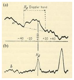
Figure 3Example of Hβ line Doppler-shifted towards the violet (a) in comparison with the unshifted line (b) observed in Vegard's laboratory.
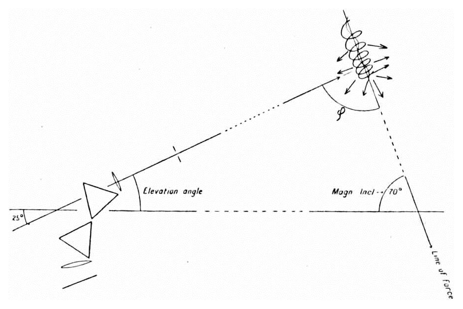
Figure 4Schematic illustrating spectral results seen by two observers looking at the same Hβ emission source, parallel and perpendicular to the Earth's magnetic field.
An energetic proton can pass through several charge-exchange cycles during an encounter with the ionosphere. The re-ionization process (2) is more likely to occur at relative low particle energies (Omholt, 1971).
On the night of 18–19 August 1950, Meinel (1950) observed extensive auroral events over the Yerkes Observatory in Wisconsin. During these events the Kp index reached 9. Data presented in Fig. 5 show a pronounced blue shift in Hα zenith observations when compared to observations in the horizontal direction. According to Meinel (1950), Vegard's observed Doppler shift on 23 February 1950 “was not outside the error margin for line identification, and thus could not be quantified”. Since Meinel had not yet seen all Vegard's spectrograms, his assertion does not represent a data-based conclusion. Vegard's measurements showed clear shifts towards the violet portion of the visible spectrum (Vegard, 1948, 1950).
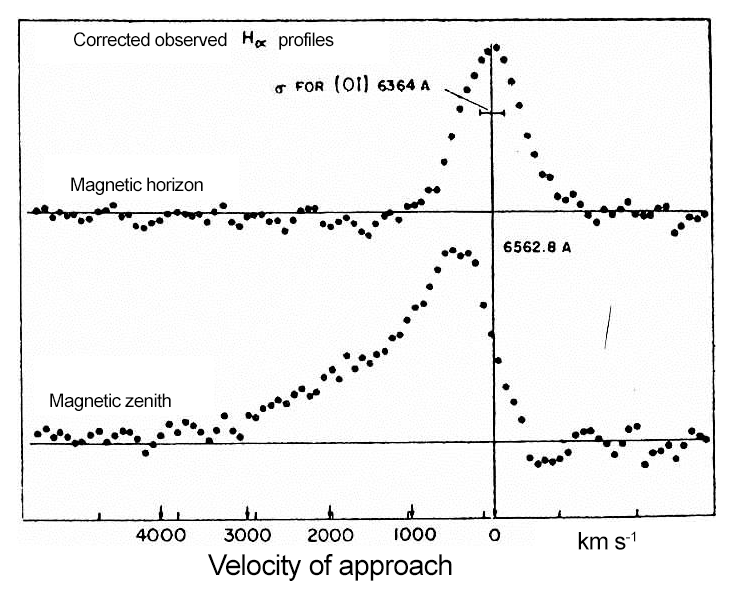
Figure 5A Doppler shift of the Hβ line towards the violet measured in kilometers per second during an intense aurora on 19 August 1950. According to Meinel (1950), the observed shift of more than 7 nm corresponds to a proton velocity of 3200 km s−1.
Figure 6 shows data acquired by Gartlein (1951) at the Cornell University Observatory in Ithaca, NY, that records a similar pattern of shifts in Hα emissions during a disturbance event (Kp=5) on 30 September 1950. A spectrograph station located at Arnprior, Ontario, ∼330 km north of Ithaca, monitored the same event. Telephone communications assured that simultaneous observations were made while looking at the same part of the arc. An Hα broadening of 1 nm in trace 2 indicates a speed of 450 km s−1 along the line of sight. From trace 4 in the figure, Gartlein estimated mean and maximum shifts of 1.5 nm and ≥3 nm, respectively. They correspond to mean and maximum speeds of 675 and ≥1350 km s−1.
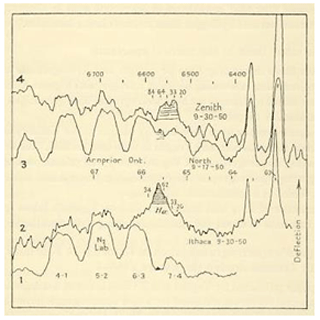
Figure 6Example of violet shift and broadening of the Hα line observed simultaneously from Ithaca, NY, and Arnprior, Ontario, during an auroral event on 30 September 1950 (Gartlein, 1951).
Based on observations made in the 1950s and 1960s, Omholt (1971) reported several events that contained violet-shifted Hα lines near local zenith that were broadened when viewed near the horizon. Most ground-based observations from that time supported the view that Doppler profiles, and hence the average energies and pitch angle distributions, did not vary drastically from one proton event to another (Omholt, 1971).
The discovery of Doppler shifts opened a new window for understanding the generation of northern lights, before the space age. Hydrogen line emissions in the northern lights could be used as proxy speedometers. Doppler shifts of the lines allow estimates of precipitating proton speeds. The larger Hα shifts towards the violet the greater the initiating proton's speed.
Hα and Hβ emissions in the northern lights are relatively weak and cannot be seen with the naked eye. Being sub-visual, long integration times may be needed while recording them, even with current technologies. Auroral emissions become visible to the naked eye only when their intensities approach 1 kilorayleigh (1 kR) (Vallance Jones, 1974; Omholt, 1971). By contrast, the very strongest Hα emissions seldom reach half that level.
Chamberlain (1961) has given a theoretical relation of the Hα and Hβ photon emission rates versus proton energy. Statistical studies show that Hα emissions are 3 to 5 times more intense than those of Hβ. Recently, Galand et al. (2004) measured the ratio to be 2.4, with an estimated rms uncertainty of ∼50 %. However, during some events, they found ratios between 1.5 and 8. The ratio varied from one event to the next, depending on the energy fluxes of precipitating protons.
Some scientists have concentrated on pure proton auroral events when hardly any electrons are involved in generating the emissions. Spectroscopically, they occur when the ratio between the intensities of the first negative band of at 427.8 nm and Hα falls to less than 3. When precipitating electrons dominate auroral processes this ratio often exceeds 10. Thus, this ratio allows a simple way for ground observers to distinguish remotely between auroral processes dominated by precipitating protons and electrons. Due to significantly weaker background contamination, contemporary observers tend to concentrate on Hβ emissions.
In 1942 Gartlein (1952) initiated a decade-long survey of hydrogen emission observations, as seen at Ithaca, New York. His observatory was further removed from the auroral oval than Vegard's sites. Gartlein's annual statistics for the 1942–1951 period, shown in Fig. 7, indicate occurrence rates with annual variation ranging between 13 and 3 events in 1947 and 1945, respectively. The total number of events during this decade was 77. Today, it is surprising that higher annual detection rates were not recorded.
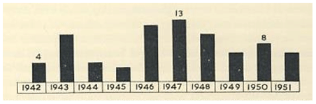
Figure 7The diagram of Gartlein (1952) for the frequency of hydrogen line detections in the aurora between 1942 and 1951.
Around 1940, Vegard noted that the occurrence frequency for detecting hydrogen lines was sporadic. During the space age, with better recording technologies and more information about where to look, weaker hydrogen lines are observed regularly in northern lights. Of historical interest, we note that after the 1970s, numerous measurements of hydrogen emissions were conducted, under both night and day conditions. The present survey considers observations acquired under both darkened and sunlit conditions.
Since the mid-1970s, detailed in situ information has become available about the dynamics and spatial distributions of energetic charged particles in the magnetosphere and the high-latitude ionosphere. Vegard's first detections of the hydrogen emissions in 1939 occurred equatorward of most electron aurorae, in the pre-midnight magnetic local time (MLT) sector.
Their different geometrical and spectral manifestations make it possible to distinguish between aurorae caused primarily by electrons and protons. As seen – particularly during nighttime – the electron-dominated aurorae show narrow structures and distinctive distributions. Conversely, proton aurorae tend to be more diffuse in form and cover larger areas. The hydrogen lines may thus appear as wide arcs.
Also, proton aurora seems to generate a continuous oval of light, stretching in the magnetic east–west direction (Omholt, 1971). The spatial domains of proton and electron auroral ovals have both considerable overlaps and separations. Before magnetic midnight the Hβ oval spreads equatorward, and peaks in intensity equatorward of the electron-generated green line. After magnetic midnight the hydrogen emissions are mainly observed poleward of the electron oval (i.e., MLat>70∘), as illustrated in Fig. 8. However, the latitude distributions depend on the energies of precipitating protons.
Figure 8b shows average spatial distributions of nightside Hβ and oxygen green line (557.7 nm) emission patterns, plotted on a MLat versus MLT grid. The optical data summarized in this plot were accumulated during magnetically active periods in the 1950s and 1960s (Omholt, 1971). For later consideration, we note that in this representation Hβ emissions may appear to be dominant over electron-caused aurora at high latitudes in the post-midnight MLT sector. The satellite image shown in Fig. 8c shows great overlap with what was observed from the ground.
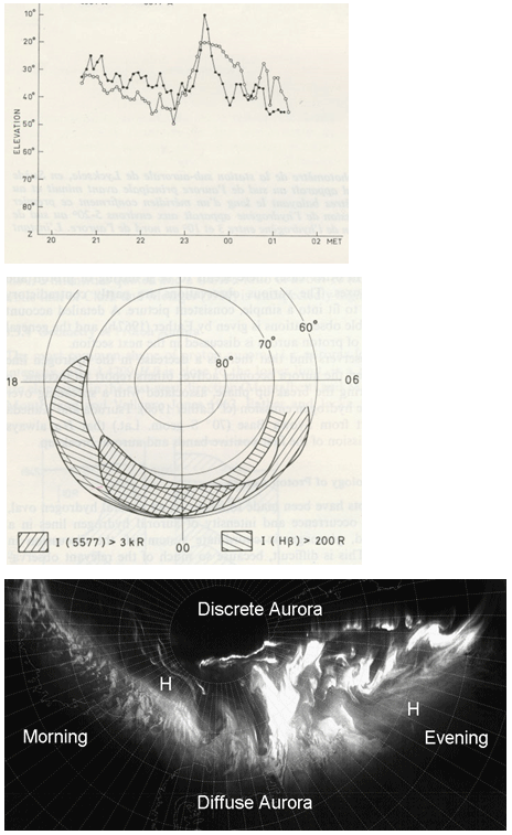
Figure 8(a) Elevation angles with respect to local zenith (∘) and intensities of the auroral green line at 557.7 nm (closed circles) and Hβ emissions (open circles) plotted as functions of mean European time (MET) for the night of 19–20 March 1966. Magnetic midnight is close to 23 MET. Data were recorded in northern Scandinavia, close to the rocket range at Andøya, under disturbed magnetic conditions (Omholt, 1971). (b) Average pattern of Hβ aurorae with intensities >200 R and electron (557.7 nm) aurora during disturbed magnetic activity (Kp>4) projected onto a magnetic latitude versus magnetic local time grid. The plots summarize nightside photometric and spectrometric data accumulated over several years in the 1950s and 1960s. The crossover in latitude occurs near magnetic midnight (Omholt, 1971). (c) This synoptic image of nightside aurora shows the relative location of the hydrogen emissions – marked with H – versus the oval, in both the morning (left) and evening (right). On the evening side the Balmer radiations are equatorward of the electron aurora, while on the morning side (left) the opposite is the case (courtesy of C. S. Deehr).
Rocket-based measurements produced the first accurate altitude profiles of the hydrogen lines as well as the downward energy fluxes and pitch-angle distributions of precipitating protons.
Because of their great horizontal extents and diffuse characteristics, accurate intensity versus altitude of hydrogen emissions can only be measured in situ. Previously Vegard (1952) and Størmer (1955) estimated that the hydrogen lines were mostly restricted to altitudes between 100 and 110 km. Altitude profiles of the hydrogen-line emissions have now been tested several times using sensors on instrumented sounding rockets. They helped quantify relationships between hydrogen-line intensities and energy fluxes of precipitating protons. We next summarize two such investigations.
The Proton 1 sounding rocket was launched at 23:30 UT on 13 February 1972 from the Andøya Rocket Range, near the Tromsø Auroral Observatory, into a nearly homogeneous auroral glow, with embedded faint structures. It reached a peak altitude of 225 km, while monitoring auroral emissions with onboard photometers. Both energy and pitch-angle distributions of precipitating particles were sampled simultaneously. Signals acquired near magnetic zenith showed both Doppler broadenings and displacements (Søraas et al., 1974).
Coordinated ground measurements by optical sensors estimated Hβ intensities of ∼170 R. Maximum Hβ emissions were identified at 112±1 km (Fig. 9) during both ascent and descent portions of the flight. Half-width emission rates were found between 107 and 119 km. The ratio of the (427.8 nm) to the Hβ emissions was ∼8, consistent with a precipitation being fairly rich in protons. Two identical rockets were launched; both recorded similar altitude profiles. They were also in good agreement with results obtained during a previous rocket flight (Miller and Shepherd, 1969).
To obtain good agreement between measured and computed Hβ profiles that accounts for the degeneration of the incoming proton beam with energies between 24 and 37 keV, as observed by Proton 1,the atmospheric density profile given in the ca. 1965 Cira model had to be reduced by a factor of 2 (Søraas et al., 1974).
The first two or three lines in the Balmer visible auroral spectrum series have been investigated since 1939. However, the OSIRIS instrument on the Odin satellites detected two additional lines. Hδ and Hε at 410.13 nm and 396.97 nm (Gattinger et al., 2010). Hε emissions lie outside the visible range. Observed intensity ratios were in agreement with published model calculations. The data reflect observations acquired in the polar region over the limb tangent altitudes between 100 and 105 km, approximately perpendicular to the Earth magnetic field. While no Doppler shifts for these new lines were recorded, observed Hα Doppler widths of 2.2 nm corresponded to H atom speeds of 500 km s−1 and average energies of ∼1.5 keV. Thus, instrumented rockets and satellites opened new opportunities to deepen understanding of proton aurora.
A large fraction of research during the first 3 decades of the space age concentrated on the plasma contents and dynamics in the near-Earth environment. Explorations focused on the solar wind/interplanetary magnetic layer (IMF), identifying different plasma regions within the magnetosphere and characterizing energetic particles and magnetic fields within the different regions. Studies of dayside air glow also proceeded with advanced optical sensors. They remotely sensed radiation coming from disparate regions in the high-latitude and midlatitude ionosphere. A new generation of meridian scanning photometers and spectrometers was deployed at the Longyearbyen and Ny-Ålesund auroral stations, Svalbard, at magnetic latitudes of 75.3 and 76.3∘, respectively. These stations are in darkness for 24 h a day between early November and late February, and are ideally located for monitoring optical radiation emitted from ionospheric projections of the dayside plasma sheet, cusp, low-latitude boundary, and mantle (Sandholt et al., 2002; Lorentzen and Moen, 2000; Newell and Meng, 1988). Robertson et al. (2006) devised a method to remove solar contamination and thereby extract Hβ contributions from spectroscopic measurements. Fortuitously, proton fluxes measured during DMSP-F12 overflights allowed confirmation of their extraction technique. Meridian-scanning photometers at both stations sampled variations in both Doppler-shifted Balmer Hα (656.3 nm) and Hβ (486.1 nm) emissions. This allowed identification of velocity filter effects in the cusp due to merging along the dayside magnetopause during periods of southward IMF Bz (Deehr et al., 1998; Holmes et al., 2008), and along the poleward wall of the cusp while IMF Bz was northward (Frey et al., 2002).
Hydrogen radiation remains a focus of ground-based aurora investigations. These studies have been augmented with data from space-based extreme ultraviolet (EUV) imagers that have been deployed on satellites such as IMAGE, TIMED and DMSP to monitor signatures of magnetosphere–ionosphere interactions. Because EUV radiation is highly absorbed in the neutral atmosphere, investigators are assured that received signals are generated in the ionosphere below the spacecraft, uncontaminated by ground interference. The IMAGE satellite has proven to be productive for understanding dayside proton aurorae and their sources. Its payload contains spectrographic imagers centered on the 121.8 nm line of H and the 135.6 nm line of atomic oxygen (OI), as well as a wideband imaging camera (WIC) sensitive to radiation in the Lyman–Birge–Hopfield band of N2 (Mende et al., 2000). Their combined data outputs allow investigators to distinguish between the contributions of electrons and protons in the auroral emissions.
In the context of investigating proton aurora on the dayside, two relevant IMAGE achievements stand out. The first concerns Lyman α emissions observed in the cusp during periods of northward IMF Bz. Consistent with ground measurements reported by Frey et al. (2003), Doppler-shifted signals indicate time-of-flight, velocity dispersions with the most energetic protons impacting the ionosphere closest to the cusp's poleward boundary. This velocity dispersion effect occurs near the poleward boundary of the cusp during northward IMF intervals (Burch et al., 1980).
The second achievement concerns the first detections of dayside hydrogen flashes at sub-auroral latitudes. These detections occur subsequent to sudden increases in the solar wind's dynamic pressure impacting the magnetopause. They typically last between 5 and 10 min. At the observed locations, the causative protons are probably of residual ring-current origins following gradient curvature drift paths inside the dayside plasmapause. Prior to the sudden environmental change, proton distribution functions were anisotropic with mostly empty loss cones. Fuselier et al. (2004) suggested that the velocity–space gradient acts as a reservoir of marginally stable free energy for the generation of electromagnetic ion cyclotron (EMIC) waves. The arrival of the solar wind pulse upsets the existing marginal stabilities to generate EMIC waves that gyro-resonantly interact with protons near the loss, causing them to diffuse into it. Within a half bounce period the gyro-resonant protons reach the ionosphere, charge exchange with ambient neutrals, and generate the Lyman α photons detected on IMAGE.
To this end, our narrative has focused on remote identifications of hydrogen lines in northern lights and inferences about their height and spatial profiles drawn from measurements accumulated over 8 decades. Vegard followed Birkeland's hypothesis that the electrons and protons responsible for the aurora were of direct solar origin. However, from both theoretical and experimental perspectives, the physical processes by which such solar–terrestrial coupling might occur remained obscure (Størmer, 1955). We outline perspectives gained during analyses of plasma and magnetic fields measured by sensors flying on satellites in deep space, and theoretical reflections on their significance. Here “deep space” refers to three distinct regimes: the solar wind, magnetosphere and topside ionosphere.
We address two distinct questions. First, how do protons responsible for the hydrogen emissions gain the kinetic energies inferred from the Doppler measurements? Average kinetic energies of protons in the solar wind are about a kiloelectron volt. How did they reach energies more than 10 times that level? Second, after being energized, how do charged particles reach the ionosphere in sufficient numbers to create the observed spatial and temporal distributions of hydrogen emissions?
Prior to explorations of the solar wind by the Soviet Luna 1 and 2, as well as the US Pioneer 5 and Mariner 2 satellites, there was a good deal of speculation about physical processes underlying interactions between the solar chromosphere and the Earth's magnetic field (Obriko and Vaisberg, 2017). The alignments of cometary tails in the anti-sunward direction, rather than along their trajectories, appeared to be inconsistent with this interpretation (Biermann, 1951). To explain this observation, Parker (1958) argued, on theoretical grounds, coronal plasma can transition to supersonic flows away from the Sun. Measurements by Pioneer 5 and Mariner 2 showed plasma flows in the solar wind were indeed supersonic. Consequently, solar wind encounters with the Earth magnetic field compress it on the dayside and stretch into a long tail-like structure on the nightside (Parker, 1968). Average speeds of protons in the solar wind are ∼400 km s−1, which corresponds to an energy of ∼1 keV. During intense storms, solar wind speeds may approach 1000 km s−1. Thus, further energization must occur to reach the tens of kiloelectron volts proton energies inferred from observed Doppler shifts of Hα and Hβ lines and their altitude profiles.
Pioneer 5 measurements also revealed the existence of an interplanetary magnetic field (IMF) embedded within the solar wind (Coleman et al., 1960) that Ness and Wilcox (1964) regarded as being of solar origin. Dungey (1961) argued that many features of auroral dynamics, such as high-latitude convection, become intelligible when the IMF has a southward component. As a solar wind parcel advects to the magnetopause, the embedded IMF and the Earth's field may be ∼180∘ out of phase. In such cases, the two fields merge. Dungey (1961) suggests the existence of three magnetic topologies: (1) interplanetary field lines with both “feet” in the interplanetary medium, (2) closed magnetic field lines with both feet attached to Earth, and (3) open field lines with one foot tied to Earth and the other in the interplanetary medium. At some distance downstream in the magnetotail, open field lines reconnect and thrust captured solar wind plasma earthward moving along newly closed field lines.
The distant magnetotail has the properties of a thin current sheet because scale sizes of magnetic field gradients in the current sheet may be comparable to or smaller than local ion gyro-radii. Thus, conditions for conserving the first adiabatic invariant breakdown, as energetic charged particles follow complex trajectories (Sergeev et al., 1983). Ions are both energized and isotropized during encounters with the cross-tail electric field (Speiser, 1967). When such ions escape from the current sheet they can reach high latitude at the nightside auroral oval. As long as the current sheet is maintained, the energetic proton populations are continuously isotropized and maintain access to the conjugate auroral ionosphere where they produce hydrogen emissions (Newell et al., 1988, 1996).
As charged particles convect earthward into the central plasma sheet (Vasyliunas, 1968), the Earth's main field on the nightside becomes more dipolar and particle trajectories more regular. Here the first adiabatic invariant is maintained and little proton precipitation is observed. However, further energization occurs in the plasma sheet via gradient-curvature drifts, to the east for protons and to the west for electrons, across equipotentials.
As energetic particles drift closer to Earth, the corotation and the convection velocities attain similar magnitudes, creating an azimuthal stagnation region. Near the dusk meridian, there is a point in the equatorial plane where the convection and corotating electric fields exactly cancel (Ejiri, 1978). The associated equipotential surface surrounding Earth, with the potential associated with this E field null point, is called the zero-energy Alfvén boundary (ZEAB). Roughly, it is collocated with the plasmapause. In the midnight local time sector, the corotation and gradient-curvature drifts for electrons are in the same westward direction. Consequently, electrons cannot penetrate closer to Earth than the zero-energy Alfvén boundary. The opposite is true for protons whose corotation and gradient-curvature drifts are oppositely directed. Ejiri (1978) showed that the convection electric field allows protons with sufficient kinetic energies to cross this boundary in the late evening sector to form the ring current, with the energy distributions sampled by the Explorer 45 satellite (Smith and Hoffman, 1974). Trajectories of plasma sheet electrons can never penetrate the ZEAB. Simultaneous measurements from the Defense Meteorological Satellite Program (DMSP) and Combined Release and Radiation Effects (CRRES) satellites during magnetic storms have independently confirmed Ejiri's conjecture (Huang et al., 2005, 2008).
The fact that satellites in high inclinations observe protons with energies of a few tens of kiloelectron volts precipitating in the dusk sector of the ionosphere, where proton aurorae are observed during magnetic storms, indicates that some physical process is operating to break the first adiabatic invariant. Otherwise, after a single bounce period the atmospheric loss cone would be empty and no ring-current protons would mirror below ∼120 km. Within a few seconds, Balmer radiation would cease. This conclusion contradicts the observations that can last for hours.
Kennel and Petschek (1966) and later Jordanova et al. (2001) argued that an emptied loss cone creates an anisotropy in the distribution functions of energetic electrons or protons. They considered the effects on particles with the pitch angles just outside the loss cone, while passing through regions in which whistler (for electrons) or ion-cyclotron (for protons) turbulence is present. If particles moving along a magnetic field line encounter waves that are Doppler-shifted to their local gyro-frequencies, the waves and particles interact strongly. The adiabatic invariant of gyro-resonant particles is then broken, allowing them to diffuse toward the previously empty loss cone; i.e., they migrate closer to the local field line's direction. In the process of migrating to the loss cone, resonant particles give up small amounts of energy to the waves, effectively amplifying them. In the proton aurora case, the process is self-sustaining as long as energetic plasma sheet protons convect across the ZEAB; they maintain the storm-time ring current with its associated proton aurora.
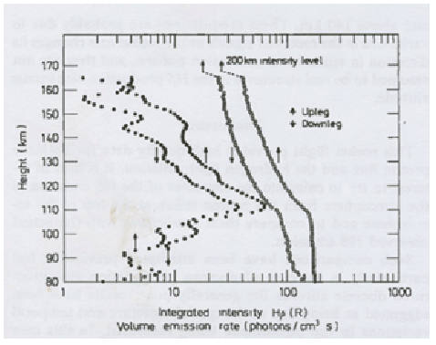
Figure 9The Hβ intensities measured by the Proton 1 rocket photometer during its ascending and descending trajectories. Some reduction in intensity appeared on the way down. Peak emissions were detected at the same altitude. Integrated intensities, recorded during the up and down legs, are shown to the right (Søraas et al., 1974).
The Balmer lines in northern lights result from excited hydrogen atoms produced when energetic protons bombard the upper atmosphere. As the precipitating protons penetrate deeper into the atmosphere, they are converted, via charge exchange, to excited H* atoms that in turn emit photons of Balmer series frequencies. Figure 10 illustrates how energetic H atoms can be re-ionized through collisions with atmospheric gases. The process repeats until bombarding protons achieve thermodynamic equilibrium with the ambient ionosphere–thermosphere. This model has successfully been used to reproduce the observed auroral hydrogen emissions, Doppler broadening and shifts (Eather, 1967; Omholt, 1971). The intensities and Doppler shifts of auroral hydrogen emissions are thus indirect measures of incoming proton energy and number fluxes. In addition, its spatial and temporal distributions provide information about their relationships with precipitating electrons.
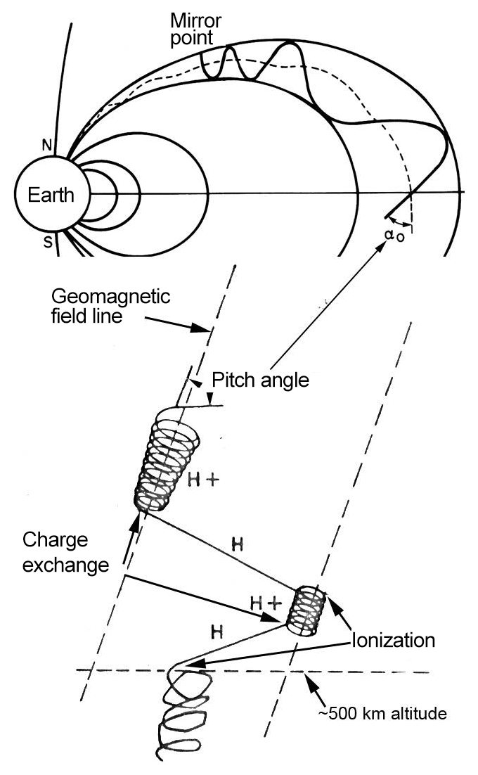
Figure 10A cartoon representation where protons bombard the Earth's atmosphere; multiple charge exchanges occur resulting in excited hydrogen atoms (H*) emissions followed by hydrogen emissions, new ionizations and charge exchanges. The production of hydrogen emissions mainly occurs below 200 km.
Most ground-based observations support the view that the Doppler profiles, and hence average energy and pitch angle distributions, do not vary drastically from one proton auroral event to another (Omholt, 1971). By comparing zenith and horizontal optical data, one can see that the hydrogen lines act as a speedometer. From the Doppler observations, we obtained the first accurate information about the velocity and energy of the precipitating auroral particles.
The nature and origins of hydrogen emissions in northern lights have evolved over the past 80 years through a remarkable synergy between laboratory-based spectroscopic experiments, ground–space observations and theoretical–numerical modeling. After many futile attempts, on the night of 18 October 1939 Professor Lars Vegard identified clear signatures of the Balmer series Hα (656.3 nm) and Hβ (486.1 nm) emissions in auroral spectra. Vegard first suggested that these emissions resulted from episodic hydrogen showers of solar origin. The third line in the Balmer series, Hγ at 410 nm, was demonstrated prior to the space age. Based on satellite observations, the Balmer Hδ and Hε lines – at 410.13 nm and 396.97 nm – as well as the extreme ultraviolet (EUV) Lyman α line at 121.6 nm of hydrogen, were also detected. From the horizon and zenith profiles one can obtain a new tool to study the precipitation of protons.
Doppler broadening and shifts provide important information about the energies of the precipitating magnetospheric protons. Both the intensities and altitude profiles of hydrogen emissions as well as their intensity ratio to the electron aurorae recorded by the first negative bands (1 NG), indicate the fraction of protons within the total precipitation. MLat and MLT distributions are also very important for understanding underlying magnetospheric processes. The hydrogen emissions often appear as a wide proton-arc oval of light. Before magnetic midnight the Hβ oval spreads equatorward of the electron-generated aurorae. After magnetic midnight the hydrogen emissions are mainly observed poleward of the electron oval. This shift in location of the proton precipitation versus MLT has also been observed by satellites.
Subsequent observations between 1940 and 1960 revealed Doppler broadenings of the hydrogen emissions. As the lines often were much broader than other atomic emissions, several scientists doubt they could come from atoms. Later confirmation of Doppler shifts came from measurements at the Yerkes Observatory during the magnetic storm of 18–20 August 1950 when a spectrograph was alternately pointed southward and northward towards the magnetic zenith and horizon, respectively. Doppler-shifted spectra were broadened while looking toward the horizon, and shifted toward the violet while looking toward magnetic zenith. Observed shifts toward the violet indicated that the field-aligned emitting protons had energies up to ∼50 keV. This is consistent with satellite measurements of storm-time proton energies in the conjugate ring current.
Space data from satellite-borne sensors made two significant contributions. (1) Energetic particle detectors demonstrated the existence of regions in the magnetosphere, conjugate to nightside proton aurorae, where conditions for breaking the first adiabatic invariants of kiloelectron volts protons prevail, allowing them to precipitate through continuously refilled atmospheric loss cones. (2) EUV imagers showed that dayside hydrogen emissions appear in response to changes in either the solar wind's dynamic pressure or the interplanetary magnetic field's north–south component.
In response to these observational challenges, the 1960s and 1970s were marked by multiple studies of cross sections for H+ <=> H charge exchange and electron stripping events needed to explain both the physical and velocity space widths of observed hydrogen emissions. The presentation outlined the development of pre-space-age understanding and modeling of proton aurorae as precise measurements by ground sensors, sounding-rocket and satellite-based sensors became available in the 1990s and beyond.
A lot of the data used have been collected by different researchers at the University of Oslo. All data from North America and other countries can be found in the cited literature; see the reference list.
AE was mainly responsible for the historical observations, while WJB presented the satellite data. WJB is also the key person together with AE for the interpretation of the observations.
The authors declare that they have no conflict of interest.
This paper was edited by Sam Silverman and reviewed by S. Okano and Finn Soraas.
Ångstrøm, A. J.: Recherches sur le Spectre Solair, Spectre Normal du Soleil, Imprimeurde d'Universite, Uppsala, Sweden, 1868.
Babock, H. D.: A study of the green auroral line, Astrophys. J., 57, 209–221, 1923.
Biermann, L.: Kometschweife und solare Korpuskularstrahlung, Z. Astrophys, 29, 274–286, 1951.
Bohr, N.: On the Constitution of Atoms and Molecules, Part I, Philosophical Magazine, 26, 1–24, https://doi.org/10.1080/14786441308634955, 1913.
Bohr, N.: On the Constitution of Atoms and Molecules, Part II Systems Containing Only a Single Nucleus, Philosophical Magazine, 26, 476–502, 1913.
Burch, J. L., Reiff, P. H., Heelis, R. A., Spiro, R. W., and Fields, S. A.: Cusp region particle precipitation and ion convection for northward interplanetary magnetic field, Geophys. Res. Lett., 97, 6369–6372, 1980.
Chamberlain, J. W.: Physics of aurora and airglow, Academic Press New York and London, 1961.
Coleman, P. J., Sonett, C. P., Judge, D. L., and Smith, E. J.: Some Preliminary Results of the Pioneer V Magnetometer Experiment, J. Geophys. Res., 65, 1856–1857, https://doi.org/10.1029/JZ065i006p01856, 1960.
Davidson, G. T.: Expected spatial distribution of low-energy protons precipitated in the auroral zones, J. Geophys. Res., 70, 1061–1068, 1965.
Deehr, C. S., Lorentzen, D. A., Sigernes, F., and Smith, R. W.: Dayside auroral hydrogen emission as an aeronomic signature of magnetospheric boundary layer processes, Geophys. Res. Lett., 25, 2111–2114, https://doi.ore/10.1029/98GL01535, 1998.
Dungey, J. W.: Interplanetary magnetic field and the auroral zone, Expected spatial distribution, Phys. Rev. Lett., 6, 47–48, 1961.
Eather, R. H.: Auroral proton precipitation and hydrogen emissions, Rev. Geophys. Space Phys., 5, 207–285, 1967.
Egeland, A. and Burke, W. J.: Kristian Birkeland, The First Space Scientist, Springer, 2005.
Egeland, A. and Burke, W. J.: Carl Størmer, Auroral Pioneer, Springer, 2012.
Egeland, A. and Burke, W. J.: Auroral research at the Tromsø Northern Lights Observatory: the Harang directorship, 1928–1946, Hist. Geo Space. Sci., 7, 53–61, https://doi.org/10.5194/hgss-7-53-2016, 2016.
Ejiri, M.: Trajectory traces of charged particles in the magnetosphere, J. Geophys. Res., 83, 4798–4810, 1978.
Franke, H.: Lexikon der Physik, 3rd ed., Franchksche Verlag, Stuttgart, 1969.
Frey, H. U., Mende, S. B., Immel, T. J., Fuselier, S. A., Claflin, E. S., Gérard, J.-C., and Hubert, B.: Proton aurora in the cusp, J. Geophys. Res., 107, 1091–1106, https://doi.org/10.1029/2001JA900161, 2002.
Frey, H. U., Immel, T. J., Lu, G., Bonne, J., Fuselier, S. A., Mende, S. B., Hubert, B., Ostgaard, N., and Le, G.: Properties of localized, high latitude, dayside aurora, J. Geophys. Res., 108, https://doi.org/10.1029/2002JA009332, 2003.
Fuselier, S. A., Gary, S. P., Thomsen, M. F., Claflin, E. S., Hubert, B., Sand, B. R., and Immel, T.: Generation of Transient Dayside Sub-Auroral Proton Precipitation, J. Geophys. Res., 109, https://doi.org/10.1029/2004JA010393, 2004.
Galand, M., Blumgardner, J., Pallamraju, D., Chakrabarti, S., Løvhaug, U. P., Lummerzheim, D., Lancaster, B. S., and Rees, M. H.: Spectral imaging of proton aurora and twilight at Tromsø, Norway, J. Geophys. Res., 109, https://doi.org/10.1029/2003JA010033, 2004.
Gartlein, C. W.: Transaction of the Oslo Meeting, IATME Bulletin no. 13, IUGG, 1950.
Gartlein, C. W.: Protons and the aurora, Phys. Rev., 81, 463–464, 1951.
Gartlein, C. W.: Memoires de la Societe Royale des Sciences de Liege, Vol. XII, 1952.
Gattinger, R. L., Egeland, A., Bourassa, A. E., Lloy, N. D., Degerstein, D. A., Stegman, J., and Llewllyn, E. J.: H Balmer lines in terrestrial aurora, J. Geophys. Res., 119, A09306-315, https://doi.org/10.1029/2010JA015338, 2010.
Holmes, J. M., Kozelov, B. V., Sigernes, F., Lorentzen, D. A., and Deehr, C. S.: Dual Site Observations of Dayside Doppler shifted Hydrogen Profiles, Can. J. Phys., 99, 1–11, 2008.
Huang, C. Y., Burke, W. J., and Lin, C. S.: Ion precipitation in the dawn sector during geomagnetic storms, J. Geophys. Res., 110, A11213, https://doi.org/10.1029/2005JA011116, 2005.
Huang, C. Y., Burke, W. J., and Lin, C. S.: Two observed consequences of penetration electric fields, J. Atmos. Solar-Terr. Phys., 110, A11213, https://doi.org/10.1016/j.jastp.2008.09.018, 2008.
Jordanova, V. K., Farrugia, C. J., Thorne, R. M., Khazanov, G. V., Reeves, G. D., and Thomsen, M. F.: Modeling ring current proton precipitation by electromagnetic ion cyclotron waves during the May 14–16, 1997, storm, J. Geophys. Res., 106, 7–22, https://doi.org/10.1029/2000JA002008, 2001.
Joyce, J. W.: Transactions of the Oslo Meeting, IATME Bulletin no. 13, IUGG, 1950.
Kennel, C. F. and Petschek, H. E.: Limit on stably trapped fluxes, J. Geophys. Res., 71, 1–27, 1966.
Lorentzen, D. A. and Moen, J.: Auroral proton and electron signatures in the dayside aurora, J. Geophys. Res., 105, 12733–12745, 2000.
McLennan, J. C. and Shrum, G. M.: On the luminescence of nitrogen, argon, and other gases, Proc. R. Soc. London Ser. A, 106, 505–512, 1925.
Meinel, A. B.: Evidence for the entry into the upper atmosphere of high speed protons during activity, Science, 112, https://doi.org/10.1126/science.112.2916.590, 1950.
Mende, S. A., Heetderks, H., Frey, H.U., Stock, J. M., Lampton, M., Geller, S. P., Abaid, R., Siegmund, O. H. W., Tremsin, A. S., Spann, J., Dougani, H., Fuselier, S. A., Magoncelli, A. L., Bumala, M. B., Murphree, S., and Trondsen, T.: Imaging from the IMAGE spacecraft: 2, Wideband, FUV imaging, Sp. Sci. Rev, 91, 271–285, https://doi.org/10.1023/A:1005227915363, 2000.
Miller, J. R. and Shepherd, G. G.: Rocket measurements of H beta production in a hydrogen aurora, J. Geophys. Res., 74, 4987–4997, 1969.
Ness, N. F. and Wilcox, J. M.: Solar origin of the interplanetary magnetic field, Phys. Rev. Lett., 13, 461–464, 1964.
Newell, P. T. and Meng, C.-I.: The cusp and the cleft/boundary layer – Low-altitude identification and statistical local time variation, J. Geophys. Res., 93, 14549–14556, 1988.
Newell, P. T., Feldstein, Y. I., Galperin, Y. I., and Meng, C.-I.: Morphology of nightside precipitation, J. Geophys. Res., 101, 17419–17422, 1996.
Obriko, V. N. and Vaisberg, O. L.: On the history of solar wind discovery, Solar System Research, 51, https://doi.org/10.1134/S0038094617020058, 2017.
Omholt, A.: The Optical Aurora, Springer, Berlin, 1971.
Parker, E. N.: Extension of the solar corona into interplanetary space, J. Geophys. Res., 64, 1675–1681, 1958.
Parker, E. N.: Dynamical properties of the magnetosphere, Physics of the Magnetosphere, edited by: Carovillano, R. L., McClay, J. F., and Radoski, H. R., Reidel Publ. Co., Dordrecht, 3–64, 1968.
Ratcliffe, J. A.: The formation of the ionosphere, Festskrift for Prof. Leiv Harang, Geophys. Publ., Oslo, Universitetsforlaget, 1972.
Robertson, S. C., Lanchester, B. S., Galand, M., Lummerzheim, D., Stockton-Chalk, A. B., Aylward, A. D., Furniss, I., and Baumgardner, J.: First ground-based optical analysis of Hβ Doppler profiles close to local noon in the cusp, Ann. Geophys., 24, 2543–2552, https://doi.org/10.5194/angeo-24-2543-2006, 2006.
Sandholt, P, E., Carlson, H., and Egeland, A.: Dayside and Polar Cap Aurora, Springer, 2002.
Sergeev, V., Sazhina, E. M., Tsyganenko, N. K., Lundblad, J. A, and Søraas, F.: Pitch-angle scattering of energetic protons in the magnetotail current sheet as the dominant source of their isotropic precipitation into the night side ionosphere, Planet. Space. Sci., 31, 1147–1155, https://doi.org/10.1016/0032-0633(83)90103-4, 1983.
Shuster, A.: On the origin of magnetic storms, Proc. Roy. Soc., London, 85, 44–50, 1911.
Smith. P. H. and Hoffman, R. A.: Direct observations in the dusk sector hours of the characteristics of the storm time ring current particles during the beginnings of magnetic storms, J. Geophys. Res., 79, 966–971, 1974.
Søraas, F., Lindalen, H. R., Måseide, K., Egeland, A., Sten, T. A., and Evans, D.: Proton Precipitation and the Hβ Emissions in a post-breakup auroral glow, J. Geophys. Res., 79, 1851–1859, 1974.
Speiser, T. W.: Particle trajectories in model current sheets, II: Applications to auroras using a geomagnetic tail model, J. Geophys. Res., 72, 3919–3932, 1967.
Størmer, C.: The Polar Aurora, Oxford, Clarendon Press, London, 1955.
Vallance Jones, A.: Aurora, D. Reidel, Dordrecht, 1974.
Vasyliunas, V. M.: A survey of low-energy electrons in the evening sector of the magnetosphere with OGO 1 and OGO3, J. Geophys. Res., 73, 2859–2884, https://doi.org/10.1029/JA073i009p02839, 1968.
Vegard, L.: The radiation producing Aurora Borealies, Nature, 86, 212–213, 1911.
Vegard, L.: Wavelength of the green auroral line determined by interferometer, Nature, 129, 23–24, 1923.
Vegard, L.: Hydrogen showers in the auroral region, Nature, 144, 1089–1090, 1939.
Vegard, L.: Mixed Commissions on the Ionosphere, Brussels. Transactions, and Report on recent work on ionospheric phenomena and on solar terrestrial relations, in: Emission spectra of the night sky and aurora, 82–91, Phys. Roy. Soc., London, UK, 1948.
Vegard, L.: Auroral spectrogram obtained in Oslo on February 23, Nature, 165, 1012–1013, 1950.
Vegard, L.: Doppler displacements of hydrogen lines and its bearing on the theory of aurora and magnetic disturbances, Geophys. Publ., 18, 1–15, 1952.
Vegard, L.: Composition, variations and excitation of the auroral luminescence spectra, Geophys. Publ., 19, 1–51, 1956.
Vegard, L. and Tønsberg, E.: The aurora borealis spectrum and the state of the upper atmosphere, Geophys. Publ., 13, 1–21, 1941.
- Abstract
- Origins of auroral spectroscopy
- Auroral emissions generated by energetic He ions
- Detections of hydrogen emissions
- Doppler-shifted hydrogen emissions
- Average characteristics of hydrogen emissions in northern lights
- Proton auroral distributions in magnetic latitude and local time
- Proton auroral studies with instrumented sounding rockets and satellites
- Hydrogen emissions in the dayside aurora
- Sources of proton aurora
- Concluding remarks
- Data availability
- Author contributions
- Competing interests
- Review statement
- References